Reconstruction of the Ocean Sink of Anthropogenic Carbon

Samar Khatiwala

Introduction

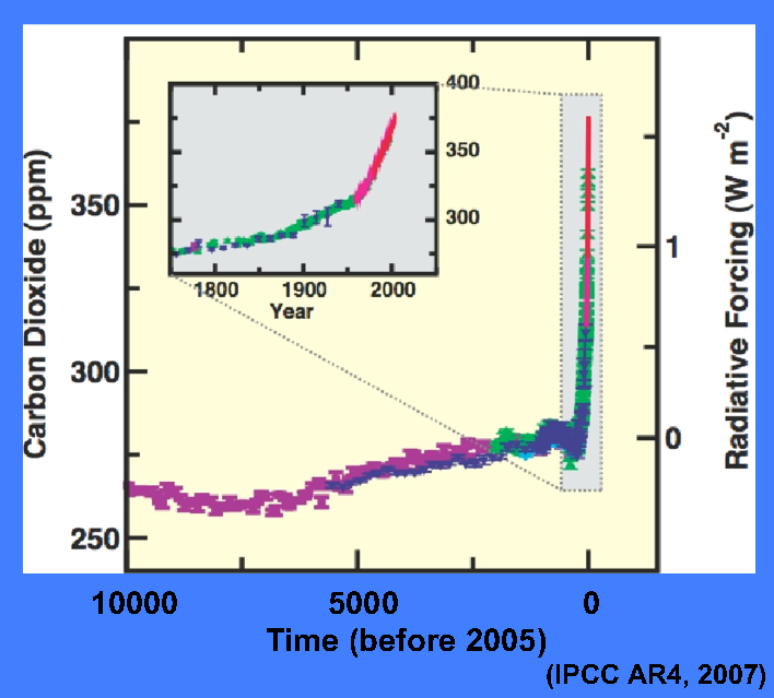
The global atmospheric concentration of CO₂ has increased dramatically as a result of human activities since 1750 and now far exceeds pre-industrial values. Indeed, present-day CO₂ levels are higher now than at any time in the past 650,000 years. The reason we care about this increase of course is because of concerns over climate change. CO₂ is a greenhouse gas (GHG). That is, it absorbs outgoing longwave radiation and thus warms the atmosphere. CO₂ is not the only GHG that is increasing due to human activity, but as the table from the IPCC report shows, its radiative effect is greater than that of all other anthropogenic GHG gases. Given the importance of CO₂ for climate, a key question is where does this CO₂ come from, and where does it go.

The cartoon below attempts to summarize our current knowledge of the sources and sinks of anthropogenic CO₂. There are two principal sources. The largest is the burning of fossil fuels which emits on the order of 8 PgC/y. (A petagram (Pg) is 1 billion metric tons.) The second largest, at around 1.5 PgC/y, is changes in land use, primarily deforestation in the tropics to make way for agriculture. Estimates for this source are relatively very uncertain however. Together, these two sources contributed somewhere between 370 to 610 PgC between the start of the industrial period (nominally taken as 1765) and 2005. So what happened to this CO₂? Less than 50% of it, or 215 PgC, currently resides in the atmosphere so the balance must have been taken up by the ocean or the terrestrial biosphere. It is believed that the ocean sequesters 20 to 35% of manmade CO₂ emissions and thus plays a critical role in mitigating the effects of this perturbation to the climate system. However, considerable uncertainties remain as to the distribution of anthropogenic CO₂ in the ocean, its rate of uptake over the industrial era, and the relative roles of the ocean and terrestrial biosphere in taking up manmade CO₂.

To address these questions, I and my colleagues, Francois Primeau at UC Irvine and Tim Hall at NASA GISS, have reconstructed the first spatially-resolved, time-dependent history of anthropogenic carbon in the ocean over the industrial era. Our work is unique in many ways. First, it is based solely on observations, and not on numerical ocean models. Second, it provides the full 3-dimensional distribution of anthropogenic CO₂ in the ocean at any instant in time between 1765 and the present. Third, our reconstruction resolves the spatial distribution of the uptake of CO₂ at the surface of the ocean, thus identifying the most intense sinks of anthropogenic CO₂ and their evolution over time. And last, the inverse method we have developed to perform this reconstruction overcomes many of the fundamental problems and limitations that have plagued previous attempts at solving this problem. Our reconstruction thus provides the first and most comprehensive view of the ocean sink of manmade carbon and, by combining with the known CO₂ emission history, the terrestrial biosphere sink. Thus, whereas before we had a single fuzzy snapshot of manmade CO₂ in the ocean, we now have a relatively sharp movie that runs from the start of industrialization to the present.

Estimating Anthropogenic CO₂ in the Ocean

The problem of estimating anthropogenic carbon (C_ant) in the ocean has challenged scientists for several decades. To understand why it is so difficult, it is useful to review some basic aspects of the problem. There are four key points to keep in mind:

Anthropogenic carbon is not a directly measurable quantity. It has to be estimated using indirect means.
The anthropogenic signal in the ocean is only a few percent of the (unknown) natural background of dissolved inorganic carbon (DIC).
Carbon in the ocean participates in rather complex in situ biogeochemistry.
Due to long transport time scales, the C_ant distribution in the ocean is highly heterogeneous.

Thus, unlike the atmosphere, which is relatively well mixed, and where we have ice core and instrumental data going back many thousands of years, the ocean is much more challenging in this regard. What we do know about C_ant in the ocean is based on so-called "back calculation" methods that attempt to separate the small anthropogenic perturbation from the large background. The essential idea, which goes back to work by Brewer, Chen, and Millero, is that we can estimate C_ant by correcting the measured total inorganic carbon for changes due to biological activity. The basic equation is shown below, where the first term is the measured DIC, the second is the change in DIC due to soft tissue remineralization and carbonate dissolution, and the third term is the air-sea CO₂ disequilibrium when the water sample was last in contact with the surface.

C_ant = DIC_meas - biological correction - air-sea disequilibrium correction …

Estimating these terms is a messy business to say the least, and it requires making several critical assumptions:

The stoichiometric or so-called Redfield ratios necessary to account for the biology are known and constant,
Mixing in the ocean is a negligible component of tracer transport compared with advection (the so-called "weak mixing" assumption), and
The air-sea disequilibrium has remained constant over the industrial era.

How valid are these assumptions? As we see below, not very. However, before we get to that, its useful to see what sort of results can be obtained with traditional inference methods. The figure below compare the results of applying three different back calculation methods to estimate anthropogenic carbon in the Indian Ocean. Clearly, while there is some qualitative agreement between them, there are large quantitative differences as well. In fact, integrated inventories differ on average by 20% between the different methods. And many of these methods, including the "ΔC*" method, which is perhaps the best known of all, give negative values of anthropogenic carbon, which points to serious problems. Lastly, back calculation methods can only provide us with a single snapshot in time. Considering that only one attempt has been made thus far to apply the ΔC* method globally (Sabine et al., 2004), resulting in an estimate for the mid-1990's, this is a perhaps one of the major limitations of this approach.

Assumption I: Redfield ratios are known and constant in space and time

A key assumption made by back calculation methods is that we know what Redfield ratios to use to correct for the biology. The difficulty with this is that there are in fact large uncertainties in our knowledge of the Redfield ratios and this translates into a correspondingly large error in the inferred C_ant. As an example, the plot below, from Wanninkhof et al. (1999), shows the fractional uncertainty in the inferred C_ant using the ΔC* method by propagating a typical (12%) uncertainty in the C:O remineralization ratio. The error is not small even for large values of C_ant. In the upper ocean, this can easily translate into a 30-50% uncertainty in the inferred C_ant.

Assumption II: Ocean transport is dominated by advection

A second implicit but crucial assumption is that ocean transport is largely advective in nature. This is an implicit assumption because back calculation techniques use transient tracers (which have a time-varying input into the atmosphere and hence the surface mixed layer of the ocean) such as CFCs to infer the time it takes for a fluid parcel to go from the surface to the interior. This works as follows. If you assume there is no mixing, then the measured interior tracer concentration is related to the surface history of the tracer through a simple time lag. If you know the surface history you can calculate the time lag. This is shown schematically in the figure on the left below.

Mathematically, we can write this as:

However, even though it underlies much of chemical oceanography, this simple picture of the ocean is fundamentally incorrect. The ocean is turbulent and diffusive, and in the presence of mixing there is no unique time scale or pathway that connects the ocean surface to an interior point. Instead, there is a multiplicity of pathways and associated transit times (see schematic on right, above), that is, a probability distribution of transit times or "transit time distribution" (TTD). Consequently, the measured tracer concentration is a weighted average of the surface history of the tracer, the appropriate weight being given by a TTD or, more generally, a Green function G, and expressed mathematically as a convolution integral:

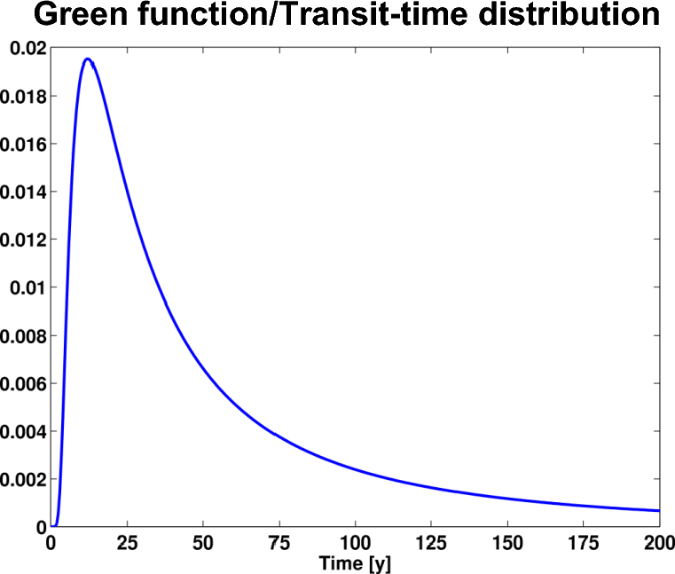
You can think of G as a way to partition each water parcel according to when and where it was last in contact with the surface. A typical example of a TTD or G is shown below. Note in particular the early peak and long tail that seems characteristic of advective-diffusive transport in the ocean. Also note that the Green function for purely advective transport would be a delta function centered at the appropriate "transit time".

There is plenty of evidence for this messier view of the ocean. As an example, the figure on the left below shows the observed relationship between two different tracers (CFC-11 and CFC-12) in the Indian Ocean. The gray dots represent data while the various curves are attempts at modeling the observed tracer distributions with TTDs (or G's) of different widths. Evidently, the data are best explained by broad G's implying strong mixing. The purely advective case (red line) is completely inconsistent with the data, something we find in other ocean basins as well.

The plot on the right shows simulations in a 1º resolution data-assimilated ocean general circulation model. (The simulations were performed using the Transport Matrix Method (TMM) developed by us, an efficient new technique for performing biogeochemical tracer simulations.) Here too, we see broad TTDs, a feature that seems independent of model resolution.

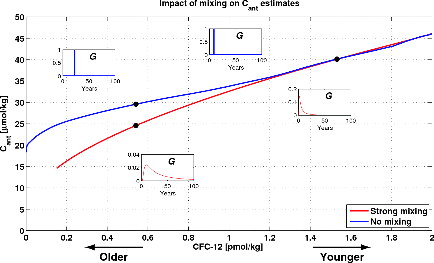
Effect of mixing on C_ant

So how does the neglect of mixing impact estimates of anthropogenic carbon? The figure below shows the inferred C_ant as a function of measured CFC-12 concentration for two scenarios. The first, shown in blue, assumes perfect advection. The second, shown in red, assumes strong mixing. You can see that in the upper ocean (higher CFC concentrations) the difference between the two is small, i.e., CFC is a good proxy for C_ant. But at intermediate depths the no-mixing assumption predicts substantially higher values of C_ant. This is because the no-mixing estimate is based on tracer ages which are biased toward younger values. Since anthropogenic carbon in the surface ocean is increasing over time, this results in a higher estimate of anthropogenic carbon in the interior. In the deep ocean, the bias is the opposite. If there is no detectable CFC, we assume that there is no anthropogenic carbon, which really cannot be true in the presence of finite mixing and the fact that anthropogenic carbon has been around for a lot longer than CFCs. Hence, this leads to an underestimate.

Assumption III: Constant air-sea disequilibrium

The third assumption is that the ocean surface has kept up with increasing levels of atmospheric CO₂. This is known as the constant disequilibrium assumption. Now, there are two main reasons why the ocean is not in equilibrium with the atmosphere. The first is the fact that it takes a finite amount of time for air-sea exchange of gases. This is about a month for most gases, but for CO₂ it is about a year because of its buffer chemistry in seawater. The second reason is ocean circulation which is continuously pumping CO₂-depleted waters away from the surface at high latitude and bringing up CO₂ enriched water in the tropics. This is why the subpolar ocean surface is highly undersaturated while the tropics are oversaturated. 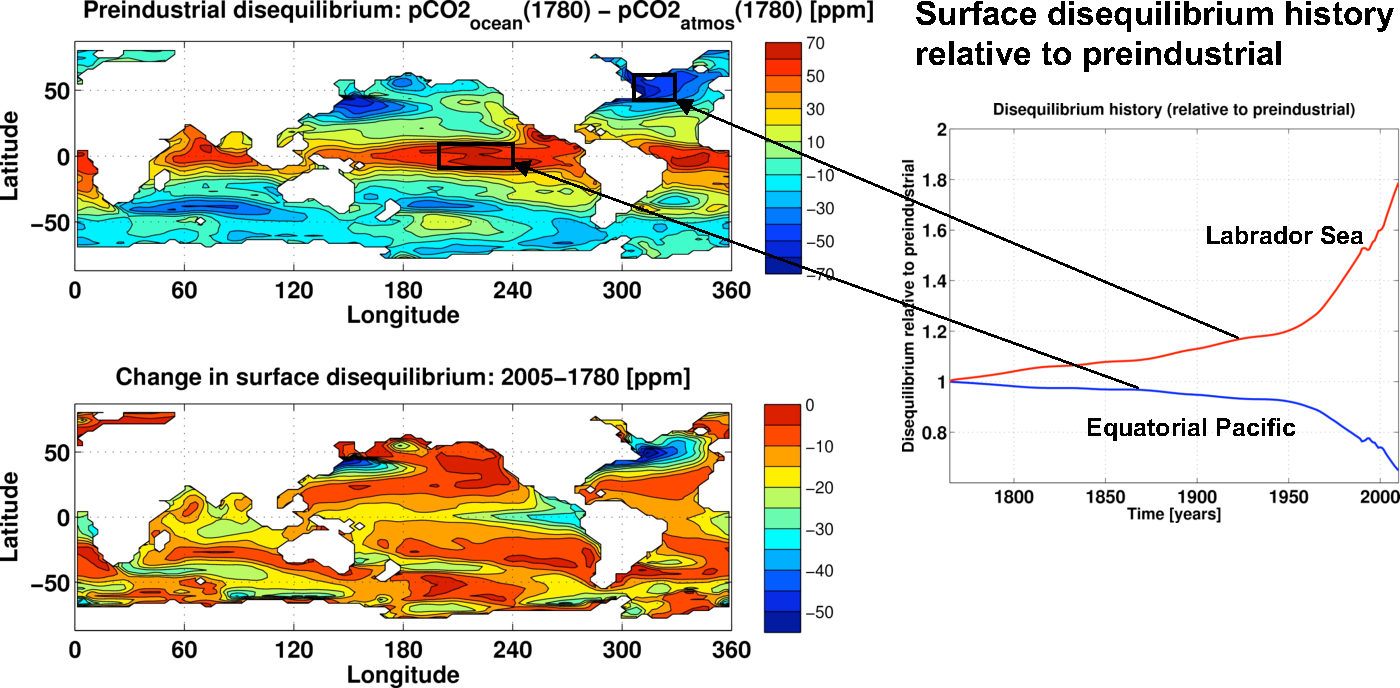The assumption is that this air-sea disequilibrium has remained unchanged over the industrial period. To evaluate how well this assumption holds, we have performed explicit simulations of anthropogenic carbon in an ocean biogeochemical model. The top right panel in the figure below shows the preindustrial disequilibrium (surface ocean pCO₂ minus atmospheric pCO₂) in the model. The bottom panel shows the change in disequilibrium between the preindustrial and 2005. It is evident that the changes are quite substantial. In fact, in the Labrador Sea the disequilibrium changes by ~80%, while in the tropical pacific it changes by ~40%. Since much of the anthropogenic carbon enters the ocean at high latitude regions such as the Labrador sea, the constant disequilibrium assumption leads to an overestimate (by almost 20%) in the estimated anthropogenic CO₂. More fundamentally, as we show below, the uptake of anthropogenic CO₂ by the ocean is in fact driven by the change in disequilibrium. Thus, assuming constant disequilibrium to estimate C_ant uptake is a contradiction.

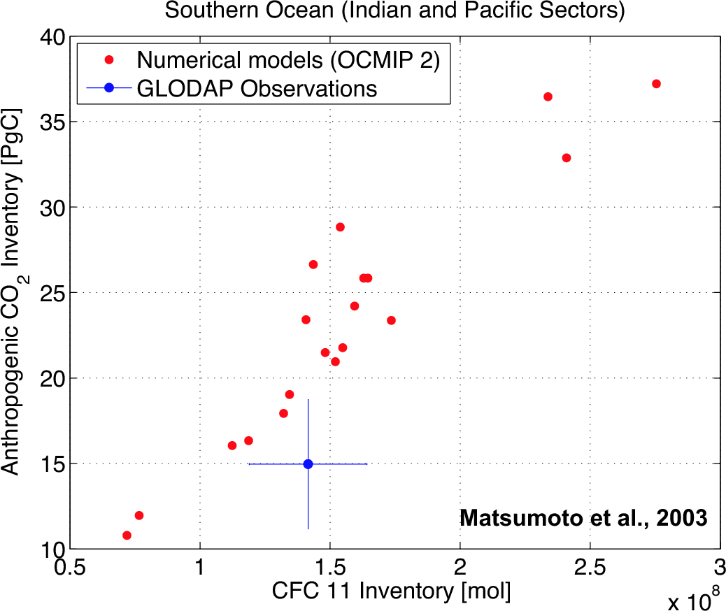
Estimates of C_ant based on ocean models

The discussion above has focused on observational-based methods for estimating C_ant in the ocean. A much simpler approach is to directly simulate anthropogenic CO₂ in coupled carbon cycle-ocean circulation models, an approach taken by a number of recent studies (e.g., Mikaloff-Fletcher et al., 2006). The problem with this approach, however, is that there is little agreement between different ocean models because they often have rather different physical circulations. In fact, as seen in the figure below, out of 19 models participating in the OCMIP-2 study (Matsumoto et al., 2003), only two managed to simulate both the Southern Ocean CFC-11 and anthropogenic CO₂ inventories within the estimated error. Certainly, over time ocean models will improve and will be essential for predicting future ocean CO₂ uptake. But first they will need to be evaluated against data-based estimates of C_ant, which as the discussion above shows remain highly problematic and limited.

A New Approach to Estimating C_ant

To overcome the problems and limitations of traditional methods for estimating anthropogenic CO₂ in the ocean, we have developed an alternative approach. In many ways it is a much simpler and cleaner approach than back calculation methods because it makes no attempt to separate the small anthropogenic component from the large background. Our method not only allows us to relax many of the (incorrect) assumptions traditionally made, it also uniquely provides us with the time-evolving spatial distribution of anthropogenic carbon over the entire industrial era. The basic ideas and assumptions are as follows:

The anthropogenic perturbation is sufficiently small for us to treat C_ant as a conservative tracer that is transported by the circulation from the surface to the interior.
Ocean transport can be characterized by a Green function.
Ocean circulation is in steady state.

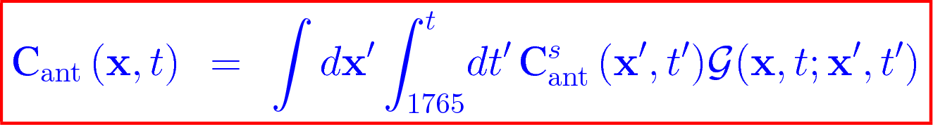
Given these assumptions, we can write the interior anthropogenic carbon concentration as a convolution of the surface history of C_ant with the Green function G:

The time integral above is over the industrial era and the space integral is over the ocean surface (since different regions will in general have different surface histories). To apply this equation, we need two pieces of information: The Green function G, and the surface history of anthropogenic carbon.

Estimating G from tracer observations

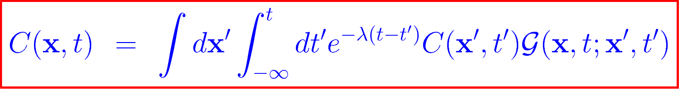
Since the Green function G is an intrinsic property of the ocean circulation, and not of any particular tracer, the concentration of any passive conservative tracer satisfies an equation analogous to that for C_ant:

We exploit this fact by using a suite of well sampled oceanic tracers such as CFCs, temperature, salinity, radiocarbon, and nutrients, to deconvolve the above equation for G. To regularize this under-determined problem we use a maximum entropy (ME) method. In practice, to reduce the indeterminancy, we assume that the ocean circulation is in steady state except for a cyclo-stationary seasonal cycle and we discretize the sea surface position variable, x', into a discrete set of surface patches. The ME solution for the i-th patch is then given by:

where M is a prior estimate of G, and α_j is the Lagrange multiplier required to enforce the j-th observational constraint. Substituting the above solution into the convolution integral for each tracer results in a small nonlinear problem whose solution is the α's.

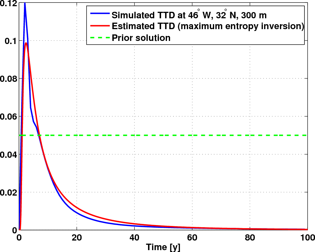
The figure belows shows a particularly successful example of the inversion. The blue line shows the directly simulated G in an ocean model. Several tracers were also simulated in the same model and the ME method was applied to these synthetic data. The red line shows the resulting ME inverse solution. The prior estimate used is shown by the green line. Here, for illustrative purposes we have used a uniform prior. In practice, we use analytical solutions to the 1-d advection-diffusion equation as priors.

Estimating the surface history of C_ant

The second piece of information we need is the surface history of C_ant. To estimate this boundary condition, we enforce mass conservation, i.e., require that the rate of change of the inventory of C_ant in the ocean be equal to its net flux into the ocean:

The air-sea flux of C_ant is in turn given by:

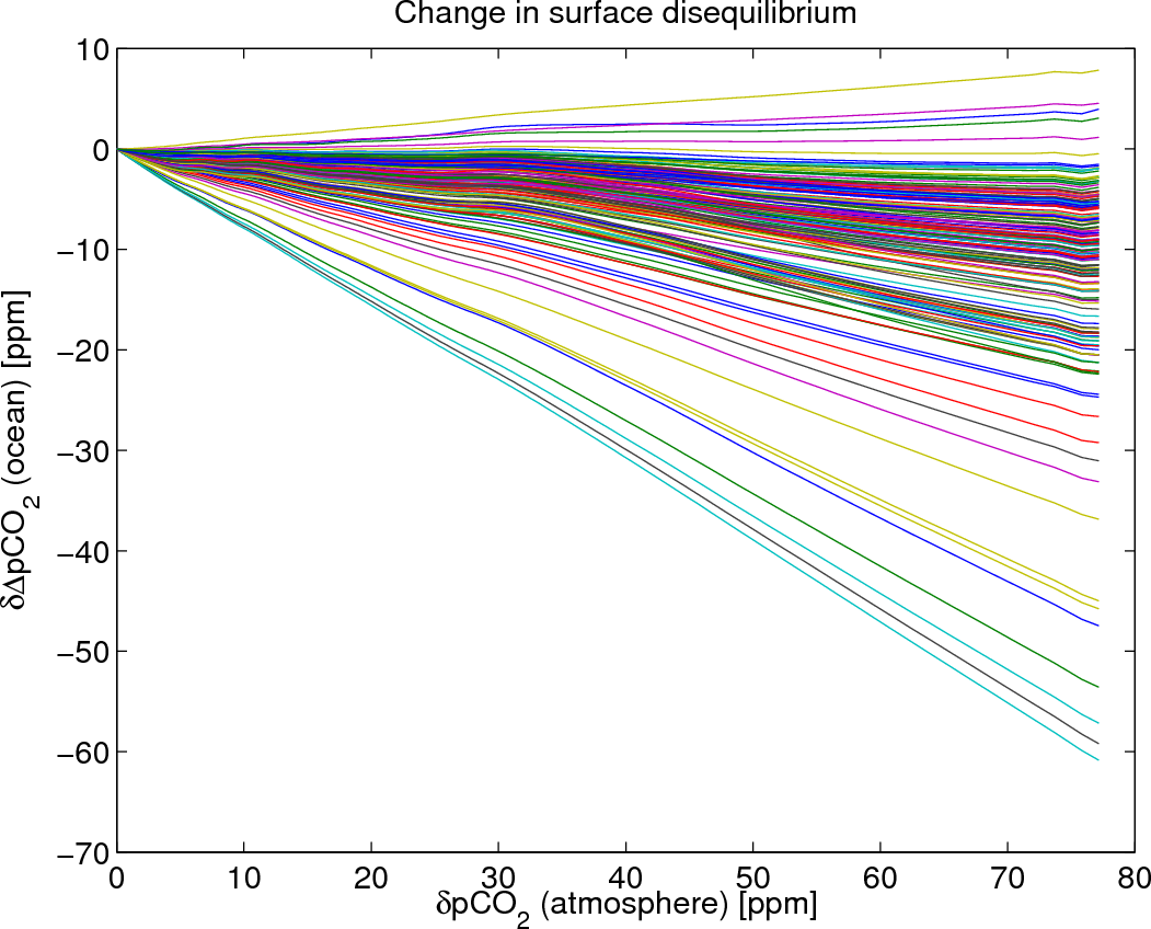
where k is a gas-transfer coefficient, D represents the air-sea difference, and d represents the anthropogenic perturbation. This equation shows that the flux is proportional to the change in surface disequilibrium of CO₂. To make further progress, we exploit the empirical result from ocean carbon cycle models (shown below from one such model) that the change in disequilibrium is to a very good approximation, proportional to the (known) anthropogenic perturbation in atmospheric pCO₂:

where e is the (unknown) proportionality constant.

Combining the above equations with the equilibrium chemistry for CO₂ in sea water, and requiring that our solution match observed pCO₂ values averaged over a discrete set of surface patches allows us to rewrite the mass conservation equation entirely in terms of e. Discretizing this equation in time and space then results in a nonlinear equation for the discrete set of e_i (one for each surface patch i). We solve it using least-squares.

To summarize, then, our inversion method provides improvements to reduce the main biases of most previous techniques. In particular,

The air-sea disequilibrium is allowed to evolve in space and time.
No assumptions are made on biogeochemical processes or parameters such as Redfield ratios.
The mixing of waters of different ages and end-member types is explicitly accounted via a Green function constrained using multiple steady and transient tracers.

Verification of Green function method in an Ocean Model

As a first step, we have applied our approach to synthetic tracer "observations" simulated in a global ocean model. Tracers simulated include, CFCs, natural ¹⁴C, nutrients, and O₂. As "truth", we also simulate anthropogenic carbon.

The figure below shows the column inventory of C_ant simulated in the model (left) and the error between the ME inverse solution and the "true" simulated solution. The agreement between the two is remarkably good, with maximum differences of O(2 mol/m²) in the Southern Ocean. The total inventory simulated in 1995 in the model is 123.7 PgC, while the inverse method gives an inventory of 125.9 PgC, an error of less than 2%.

Reconstruction of Anthropogenic CO₂ in the Ocean

Having gained confidence in our method from the synthetic inversion, we next applied it to oceanographic data. Tracers used include gridded fields of CFC-11, CFC-12, and natural ¹⁴C from the GLODAP database (Key et al., 2004), and temperature, salinity, oxygen and phosphate from the World Ocean Atlas (2005). Following Broecker et al. (1998), oxygen and phosphate are combined into a quasi-conservative tracer known as PO*. The surface is partitioned into 26 discrete patches based on sea water density. pCO₂ data required to estimate the C_ant surface boundary condition are taken from the Takahashi et al. (2009) database. Using our new inverse method on this suite of observations, we have reconstructed the first 3-dimensional, time-varying, history of anthropogenic carbon in the ocean from 1765 to 2008.

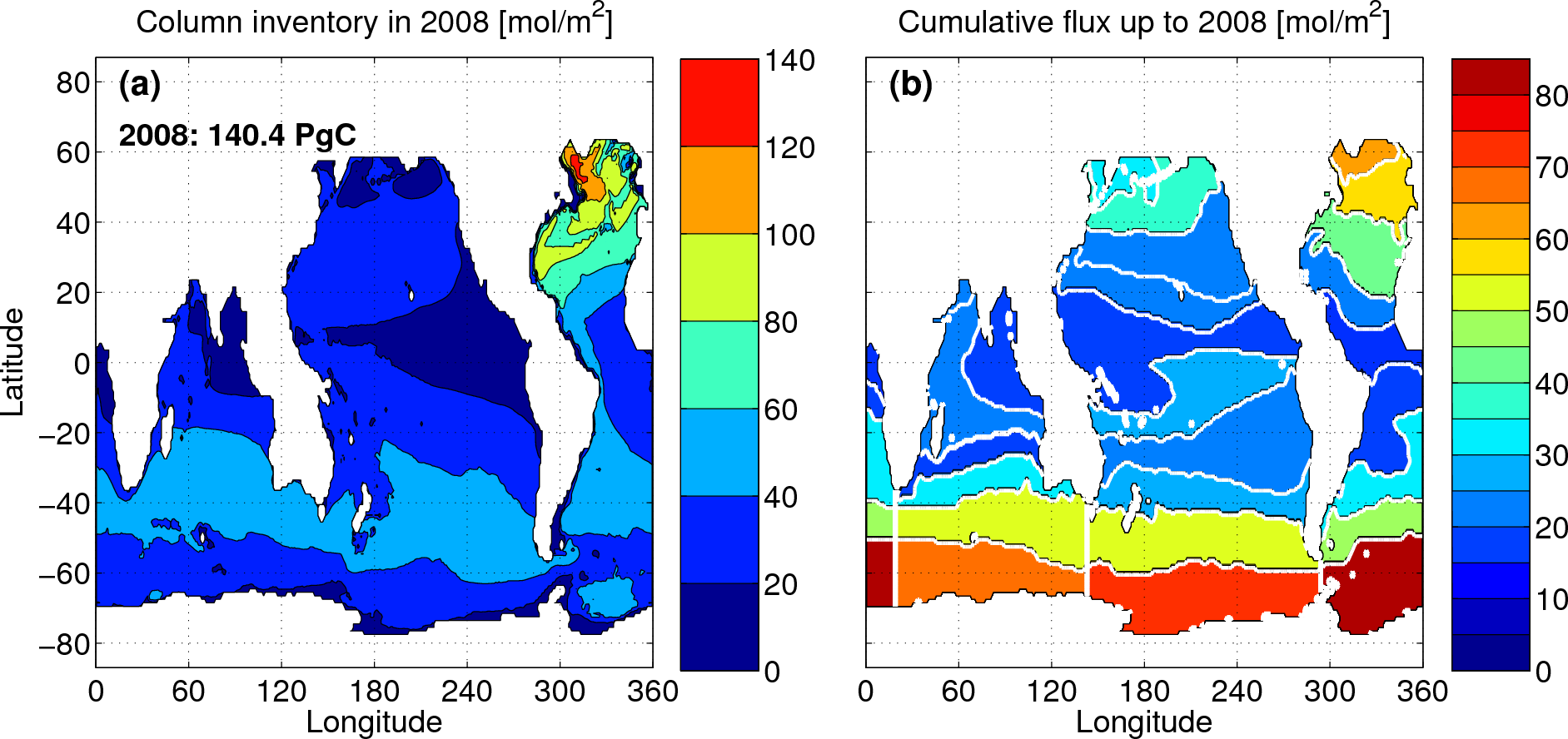
The figure on the left below shows the column inventory of C_ant in 2008. The total inventory in that year was ≈140±25 PgC. (The Arctic Ocean and marginal seas are not covered by the GLODAP database. Using the recent estimate of Tanhua et al. (2009) for the former, and the area scaling approach advocated by Sabine et al. (2004) for the latter, would increase our estimate of the global inventory by ~11 PgC.)

The animation below shows the column inventory of anthropogenic carbon over the industrial period. The movie runs from 1775 to 2007. The total inventory is shown in the upper left corner.

These are net global estimates, but, uniquely, we can go further. We can partition the uptake according to where at the surface the anthropogenic CO₂ penetrated the ocean. As is evident from the right panel in the figure above, the high latitude oceans, driven by intermediate and deep water formation, constitute the most intense sinks of C_ant. (The white lines in the figure delineate the 26 surface patches used for the inversion.) In particular, the Southern Ocean is by far the largest conduit by which anthropogenic CO₂ enters the ocean: roughly 40% of the C_ant residing in the ocean in 2008 entered the ocean south of 40ºS. Interestingly, only a small fraction of the CO₂ taken up by the Southern Ocean accumulates in that region. Much of this CO₂ is transported northward by ocean circulation. The animation below shows the cumulative uptake (in PgC) through each of the 26 surface patches. The movie runs from 1775 to 2007.

It is useful to compare our results with previous estimates of C_ant in the ocean. To date, only two global estimates of C_ant have been made. Both are snapshots for 1994. Our estimate of the global inventory in that year is 114±22 PgC, which is consistent with both the ΔC* based estimate of 106±21 PgC (Sabine et al., 2004), and the TTD-derived estimate of 107 (94-121) PgC (Waugh et al., 2006). However, the previous TTD based estimate incorrectly treated air-sea disequilibrium as constant. To account for this, Waugh et al. included an ad-hoc 20% downward correction based on numerical model simulations in their reported result. Our estimate does not require such a correction because our inverse method explicitly accounts for changing air-sea disequilibrium. While our estimate for the global inventory also agrees well with the ΔC* based estimate, the spatial distribution we obtain is quite different. In particular, relative to the ΔC* based estimate, our estimate of C_ant is generally lower in the upper ocean and higher in the deep ocean. The reasons for this can be understood in terms of the various assumptions made by the ΔC* method. In particular, two fundamental assumptions of the ΔC* are the use of a single tracer age to characterize transport (effectively assuming that ocean circulation is essentially advective) and that air-sea disequilibrium has remained constant since the start of the industrial period. As the discussion above showed, both these assumptions are incorrect, and give rise to competing biases which happen to largely cancel out, leading to the close, but fortuitous, agreement in total inventory estimated using the ΔC* method and our estimate.

So much for the inventory and distribution of C_ant. What about the uptake rate? From the time-varying inventory, we can compute the uptake history over the industrial era. The figure below shows the uptake between 1765 and 2008. As is evident, the uptake rate has changed dramatically over time. In particular, there was a sharp increase in ocean uptake since the 1950's, driven by the higher growth rate of atmospheric CO₂. It currently stands at 2.3 PgC/y, i.e., for every four tons of CO₂ that humans produce, the oceans absorb a bit over a ton.

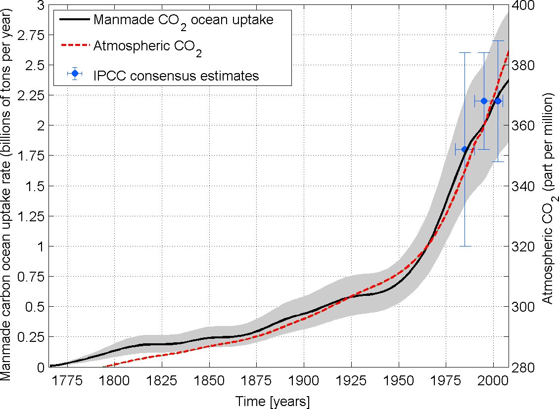
More recently, however, while the uptake rate has kept on increasing, its rate of increase appears to have slowed somewhat even though atmospheric CO₂ levels continue to increase at roughly the same rate. This seems consistent with recent evidence (Canadell et al., 2007) for an increase in the airborne fraction (the proportion of human CO₂ emissions that remain in the atmosphere), suggesting that the intensity of both the land biosphere and ocean sinks is declining. Indeed, we find that between 2000 and 2007, the fraction of emissions taken up by the ocean has declined by almost 10%. Why might this be? Since we assume a steady circulation, it can't be due to changes in ocean circulation as suggested by some recent studies based on ocean climate models. For example, Le Quere et al. (2007) claim that the Southern Ocean sink of manmade carbon is declining - in the model - because of an increase in the strength of the meridional overturning circulation in response to changes in the westerly winds. This is debatable, however, since there are both empirical and theoretical grounds for suspecting that coarse resolution ocean models - in which eddies are parameterized - do not correctly capture the behavior of the real ocean. We should also keep in mind that the rate of growth of emissions is increasing. According to Raupach et al. (2007), the growth rate of emissions has increased sharply this decade compared with the previous one. Between 1990-1999 emissions grew by 1.1% per year, while from 2000-2004 they grew by over 3% a year, almost a 3-fold increase. Taking these together, there are two plausible explanations for why the ocean uptake is slowing down relative to emissions. The first explanation is ocean chemistry. As the ocean takes up CO₂, its capacity to take up more anthropogenic carbon decreases due to the nonlinear nature of the CO₂ chemistry in sea water. This "buffering" effect is well understood. In fact, when we linearize the chemistry in our calculations, the aforementioned decline in the rate of increase of uptake reduces substantially. The second explanation is that the ocean is simply not able to 'keep up' with the rapid growth in emissions. There is a physical limit (due to air-sea gas exchange and ocean circulation) on how rapidly CO₂ can enter the ocean. If the emissions grow too quickly, then the ocean can't keep up. Indeed, we have shown recently that the airborne fraction is quite sensitive to the emission history and that a 10% increase in the rate-of-growth of emissions leads to a 3-4% increase in the airborne fraction. Thus, rather than invoking 'exotic' mechanisms such as large scale changes in ocean circulation, we believe it is basic physical and chemical factors that are limiting the ocean's ability to take up fossil fuel CO₂.

Also shown on the figure above are the IPCC AR4 "consensus" estimates. (These are decadal averages.) There is generally good agreement between our estimates (which cover the entire industrial period) with the IPCC ones (which only go back to the 1980's). In particular, our estimate for the present decade is 2.3±0.6 PgC/y, while the IPCC estimate (which is actually based on an ocean model) is 2.2±0.4 PgC/y.

Implications for the Role of the Terrestrial Biosphere in Uptake of Anthropogenic CO₂

One of the major uncertainties in our understanding of the anthropogenically-perturbed carbon cycle is the role of the terrestrial biosphere. Since direct CO₂ flux measurements, especially on a global scale, are at best difficult to make, the terrestrial source/sink term has typically been computed as a difference between the relatively well constrained source of anthropogenic CO₂ due to fossil fuel burning, and the atmospheric and ocean sinks. The difficulty with this approach is that until now only a single estimate of the inventory of C_ant in the ocean has been available (for 1994). To get around this, scientists have resorted to using numerical models of ocean CO₂ uptake to quantify the land term. However, as discussed above, this approach has its own problems, among them being the large errors in simulated transport in current ocean models, and the correspondingly large disagreement in simulated uptake between different models. Our time-evolving, purely data-based estimate of the ocean uptake allows us to circumvent these problems, and provide a more precise and detailed view of the land sink.

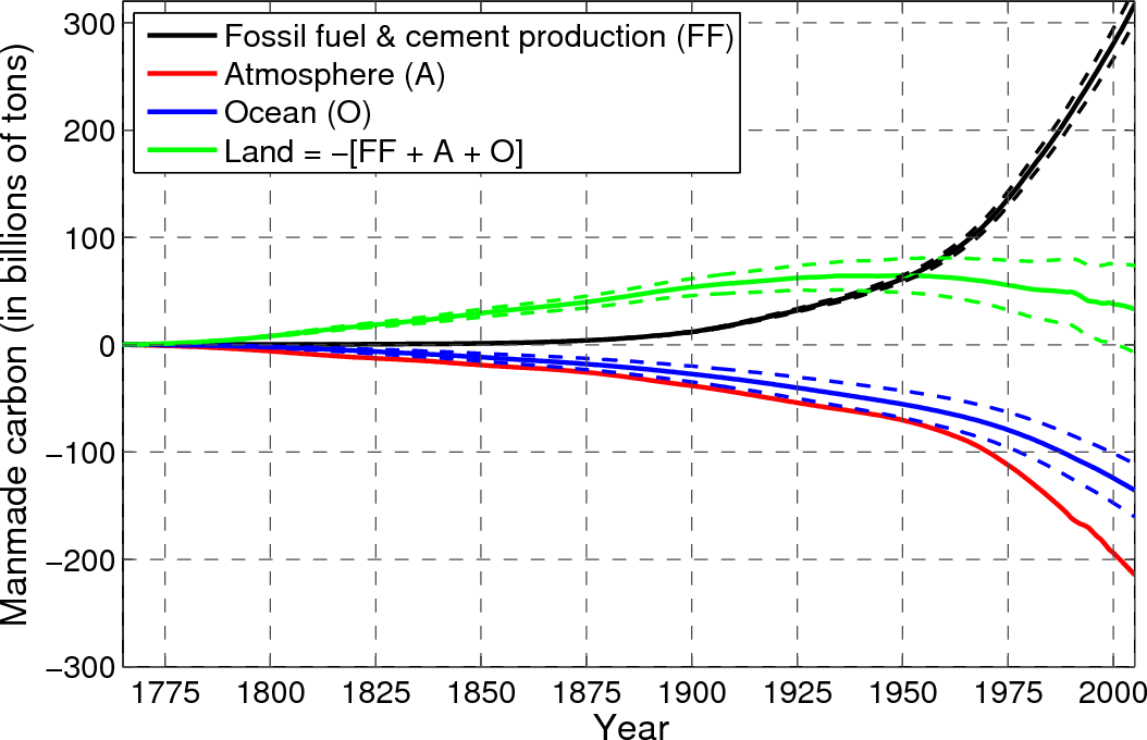
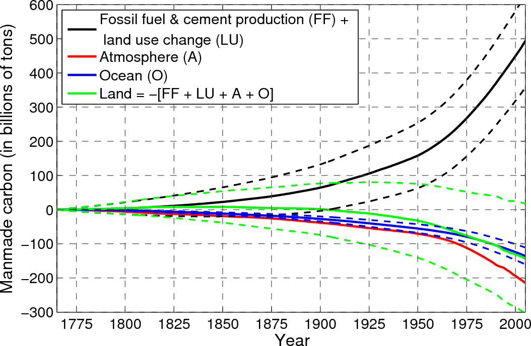
The figure below between shows the time evolution of the main fossil fuel source and the ocean and atmosphere sinks between 1765 and 2005. Also shown is the terrestrial biosphere inventory, computed as the difference between the fossil fuel source and the ocean and atmosphere. Sources are shown as positive values and sinks as negative values. Fossil fuel data are taken from Marland et al. (2007). As is evident, the terrestrial biosphere was a source of anthropogenic carbon until the 1940's, subsequently turning into a sink. Cumulatively over the entire industrial period, our best estimate is that the terrestrial biosphere was a net source of C_ant. Propagating uncertainties, we find that the terrestrial biosphere has been anywhere from neutral to a net source of CO₂, contributing up to half as much C_ant as has been taken up by the ocean over the same period.

In the discussion above, we only included fossil fuel burning as a source of anthropogenic CO₂ in the computation of the "net terrestrial sink". However, another source of C_ant is changes in land use, estimates of which, as mentioned previously, remain highly uncertain. Including this term as a source provides a different perspective on the role of the terrestrial biosphere. The figure below show the evolution of what is sometimes termed the "residual terrestrial sink" (computed as above, but including land use changes (from Houghton, 2008) as a source). Note the very large error envelope associated with this curve. Our best estimate suggests that cumulatively, the terrestrial biosphere currently contains roughly the same amount of anthropogenic CO₂ as the ocean. However, given the uncertainty, the terrestrial biosphere could be anywhere from neutral to twice as important a sink of anthropogenic CO₂ as the ocean.

Implications for Future CO₂ Uptake and Ocean Chemistry

Lastly, we explore the implications of our work for future CO₂ uptake by the ocean. As discussed above, our results suggest that changes in ocean chemistry (i.e., acidification) may already be limiting the ability of the ocean to take up more manmade CO₂. It is therefore useful to explore how continued penetration of CO₂ by the ocean will impact ocean chemistry and thus the role of the ocean as a sink of man made CO₂. As a preliminary step, we have used our Green function method to predict future CO₂ uptake in response to projections of atmospheric CO₂. As an example, the animation below shows the evolution of the aragonite lysocline depth for 4 different IPCC emission scenarios, starting with the most aggressive (A1FI) in the top left corner to the least aggressive (B2) in the bottom right. The movie runs from 2000 to 2100. The lysocline represents the surface above which CaCO₃ is able to precipitate out of seawater (and form shells). Below this surface, the water is undersaturated with respect to CaCO₃. As is evident, by the year 2100, much of the surface Southern Ocean and large parts of the North Pacific become undersaturated for the A1FI scenario (grey shading). Even in the most optimistic case (B2), we find that many parts of the surface Southern Ocean become undersaturated.

Summary

We have developed a new, purely data-based, inverse method to reconstruct the first 3-dimensional, time-varying, history of anthropogenic carbon in the ocean over the industrial period (1765-2008). Our approach overcomes many of the fundamental problems and limitations that have hindered previous attempts at solving this problem, and provides the most comprehensive view to date of the ocean sink of manmade carbon. We find a total inventory of anthropogenic CO₂ in the ocean in 2008 of ≈140±25 PgC (≈150 PgC if we include the Arctic), and a corresponding uptake rate of 2.3±0.6 PgC/y. Thus, the world's oceans currently absorbs roughly a quarter of manmade carbon. Our reconstruction quantifies the spatial and temporal distribution of where at the surface this CO₂ enters the ocean, and indicates that roughly 40% of this CO₂ penetrated via the Southern Ocean. However, only a small fraction remains in the Southern Ocean, with the bulk of it being transported northward by ocean circulation. We also find that CO₂ uptake has increased sharply since the 1950's, with a small decline in the rate of increase in the last few decades. In particular, between 2000 and 2007, the proportion of emissions absorbed by the ocean has declined by as much as 10%. There may be several reasons for this slowdown, but changes in ocean chemistry, compounded by the ocean’s slow circulation in the face of accelerating emissions, offer plausible explanations. This is in contrast to other studies, based on climate models, suggesting large scale changes in ocean circulation as a cause for the relative decline in the ocean sink. Lastly, combining our reconstruction with the known history of anthropogenic emissions, gives us a more precise and detailed view of the terrestrial biosphere sink. Our results suggest that the terrestrial biosphere was a source of CO₂ until the 1940's, subsequently turning into a sink that has averaged ≈1.1 (0.4-1.8) PgC over the past decade. Cumulatively, the terrestrial biosphere has been anywhere from neutral to a net source of CO₂, contributing up to half as much CO₂ as has been taken up by the ocean since the start of the industrial period.

Acknowledgment

This research was funded by the U.S. National Science Foundation.

Introduction

Estimating Anthropogenic CO2 in the Ocean

Assumption I: Redfield ratios are known and constant in space and time

Assumption II: Ocean transport is dominated by advection

Effect of mixing on Cant

Assumption III: Constant air-sea disequilibrium

Estimates of Cant based on ocean models

A New Approach to Estimating Cant