Now that we've got a list of the data files of interest, we want to make some quick plots to see what we've got. These will not be the prettiest plots, as none of the data has been edited. None-the-less, MB-System™ will create nicely formatted plots, even if the data is a little unpolished.

First, perhaps we'd like to look at just the navigation data and see the ship track for this survey. To do that we call mbm_plot as shown below:

mbm_plot -F-1 -I survey-datalist -N

Here, -F-1 specifies the format, in this case "-1" indicates that the input is a list of files rather than an individual file and that the format for each file is specified in the list. Of course, -I survey-datalist is our list of data files. A navigation plot is specified with -N. With this simple line, and nothing more, we get a script that will create a navigation plot with default annotations, grid lines, tick marks, etc.. The results of executing the line above are shown below.

Plot generation shellscript <survey-datalist.cmd> created.

Instructions:
  Execute <survey-datalist.cmd> to generate Postscript plot 
<survey-datalist.ps>.
  Executing <survey-datalist.cmd> also invokes ghostview to
  view the plot on the screen.

A script was created called survey-datalist.cmd. When executed the script will create the navigation plot as a post script file and then execute ghostview to view the plot immediately. When we execute the resulting script the following plot is created:

Figure 3.1. Survey Navigation Plot

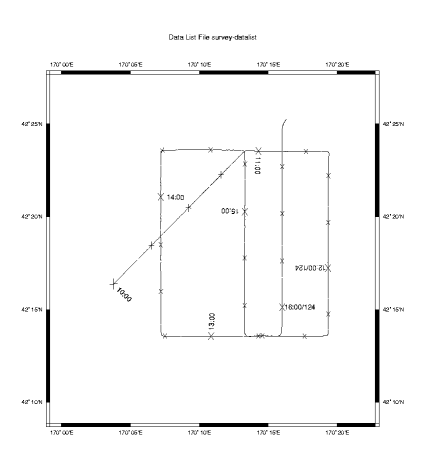
Wasn't that easy? mbm_plot sets default tick marks, grid lines, and longitude and latitude annotations as well as track annotations. It takes care of centering your plot onto a single page and even adds a title. All of these details, of course, can be changed though the myriad of options to mbm_plot. Have a look at the man page for the details.

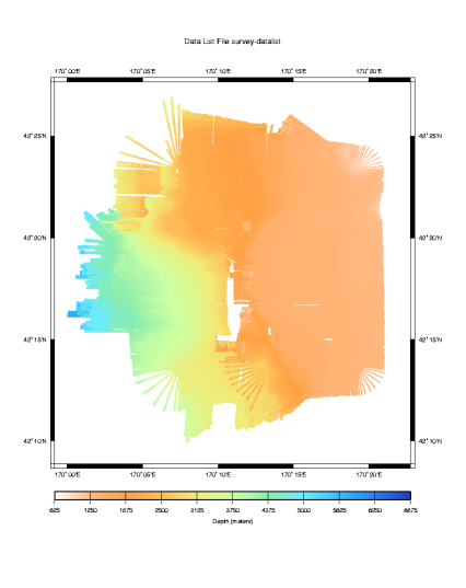
Now let us take a look at the bathymetry data itself. We might start with a color plot of the bathymetry data. One specifies plotting of the bathymetry data by indicating a "graphics" mode utilizing the "-G" flag to mbm_plot. Five graphics modes are supported:

Then to create a color fill of the bathymetry data, we execute the following:

mbm_plot -F-1 -I survey_filelist.124 -G1

Here is the resulting plot.

Figure 3.2. Color Bathymetry Plot

Now perhaps we'd like to add some contours to our color plot, and maybe add the navigation back in as well. A quick contour plot with default parameters can be specified with the "-C" flag.

mbm_plot -F-1 -I survey_filelist.124 -G1 -N -C

The resulting plot is shown below:

Figure 3.3. Color Bathymetry Plot with Contours

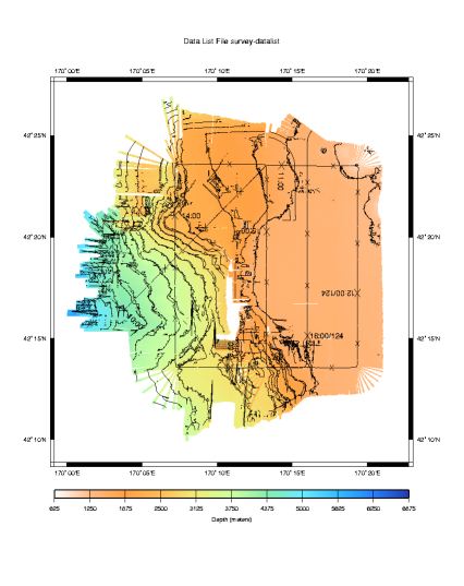
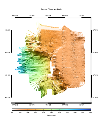
What a nice plot of the data set! We can quickly see the lay of the sea floor, maximum and minimum contours, the ship track's coverage, and oddly shaped contours here and there already give hints as to where we we might need to spend special attention in our data editing.

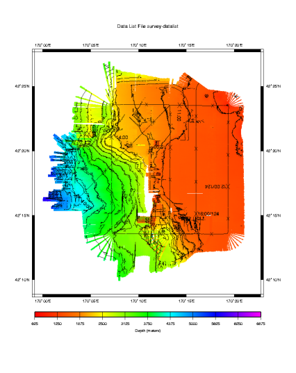
Just for fun, lets create the same plot with a different color scheme. mbm_plot has a few predefined palettes that do not require us to create our own color map. These can be specified with the "-W" flag followed by the color style (continuous or discrete intervals), and optionally the palette (1-5) and number of colors(11 default).The following will create the same plot with mbm_plot's "high intensity" color palette.

mbm_plot -F-1 -I survey_filelist.124 -G1 -N -C -W1/2

Here's the resulting plot:

Figure 3.4. High Intensity Color Bathymetry Plot with Contours

mbm_plot can also quickly create shaded relief maps. These are specified with graphics mode "2" listed above, and by default produce a plot with artificial illumination from the north. The direction of illumination may be modified with the -A flag. See "COMPLETE DISCRIPTION OF OPTIONS" in the man page for more details.

mbm_plot -F-1 -I survey_filelist.124 -G2

Here's the resulting plot.

Figure 3.5. Shaded Relief Color Bathymetry Plot

Finally we might wish to see a plot of the side scan data. Sidescan plotting is also specified by a graphics mode, in this case mode "5".

mbm_plot -F-1 -I survey_filelist.124 -G5

Here is the plot:

Figure 3.6. Sidescan Plot

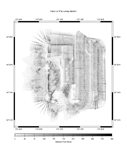
The plot above is not as nice as we might like. Much of shading is lost on erroneously high sidescan values which have incorrectly weighted the grayscales. The result is a fuzzy, washed out side scan image. This particular data set covers such a large range of side scan values (due to a change of several 1000's of meters in depth plus normal noise) that the side scan image looks quite poor. In this case, we will have to edit the data to remove the erroneous data spikes and then renormalize the gray scaling to get a good side scan image. We leave that to another chapter.

Now that we've explored the data sets graphically one might be interested to extract some statistics about the data set. This leads us to the next section.