 |
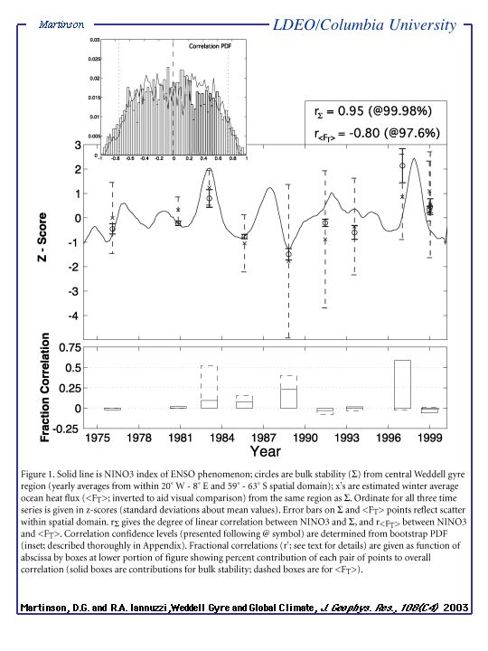 |
Figure 1 -In Figure 1, Σ (bulk stability) and < FT > (ocean
heat flux), averaged anually within a spatial domain encompassing Maud Rise... |
 |
 |
Figure 2 -Figure 2 examines the individual cruise tracks as well as the climatologies of Martinson
and Iannuzzi 1998 in an effort to locate fronts, abrupt property transitions and regions of maximum lateral property gradients;... |
 |
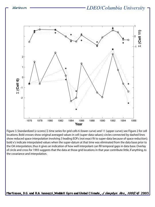 |
Figure 3 -Figure 3 gives results from two grid cells: one (cell 11) is densely sampled, the other
(cell6) is sparsely sampled. |
 |
 |
Figure 4 -Three leading EOF's lie above the noise floor for both Σ and < FT >. These EOF's and their PC's describiing 43%, 20% and 9% of the total variance for Θ and 31%, 25% and 18% for < FT >.
|
 |
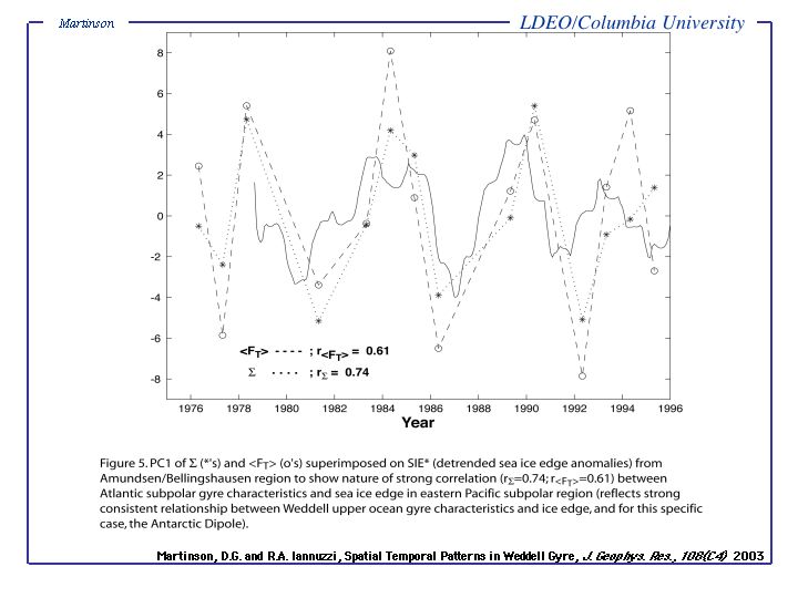 |
Figure 5 -Strong PC-SIE* correlations in the Pacific sector and Weddell gyre region. |
 |
 |
Figure 6 -Statistical assessment of the correlation maps are presented in Figure 6 via confidence
interval contours, whose derivation are described in Appendix 1*. |
 |
 |
Figure 7 -Results of correlating NINO3 to the super-data as well as the OA gridded data are
presented in Figure 7. |
 |
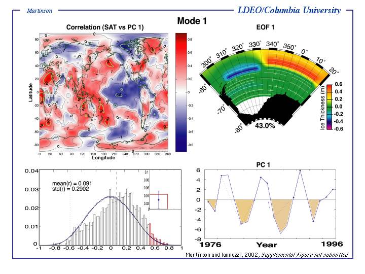 |
Mode 1 -(Supplemental figure not published)This gravest mode appears to
be a "global" mode, showing considerable covariability about the globe. |
 |
 |
Mode 2 -(Supplemental figure not published)The second mode appears to
be more clearly an ENSO realted mode though it too shows global teleconnections |
 |
 |
Mode 3 -(Supplemental figure not
published)Mode 3 shows elements of each of the two graver modes, though covariability with
the Atlantic seems to dominate, with the Indian Ocean and Mesopotamia showing strong links as well. |
)
)
)
)
)
)
)
)
)
 Home
Home