Figures

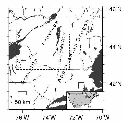
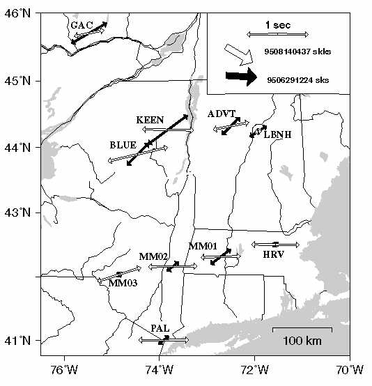
Figure 1. Map of the study area. Wide dashed line shows the transition from Grenville Orogen to the Appalachian Orogen, with the Adirondack Mountains shown in grey. (Postscript Version).

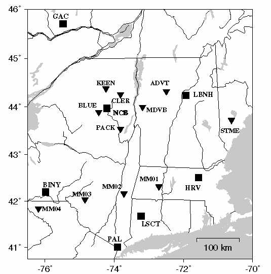
Figure 2. Seismic stations used in this study. Permanent installations (boxes) belong to US and Canadian national networks, IRIS GSN and LDEO. Temporary deployments include MOMA, ABBA and stations deployed by the authors (see Table 3). The network configuration shown was deployed during the spring and summer of 1995. (Postscript Version).

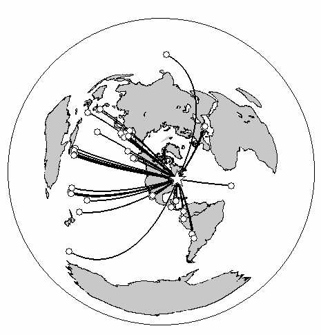
Figure 3. Locations of earthquakes recorded by the network. Events arriving from the west dominate the dataset. (Postscript Version).

Figure 4. (a) Two core-refracted shear phases observed by the network. Waveforms are corrected for instrument response and band-limited between 0.01 and 0.2 Hz. Bold lines show radial component, thin lines - transverse. (b) Map of the region showing shear-wave splitting parameters detemined for the two phases. Splitting azimuth and delay are shown at each station as arrows aligned with fast direction and scaled with delay . Splitting arrows, as well as phase vectors in the upper left, are color-coded by event, black for one and white for the other. Note that the splitting direction for the two events is quite different, yet is fairly consistent across the region for each event. (Postscript versions: Fig 4a, Fig 4b).

Figure 5. Splitting parameters obtained for all stations. Observations are shown as arrows aligned with the fast direction and scaled with delay , plotted as a function of backazimuth and phase velocity. At all stations significant differences are seen between splitting parameters obtained for different backazimuths. (Postscript versions: Fig 5.1, Fig 5.2).

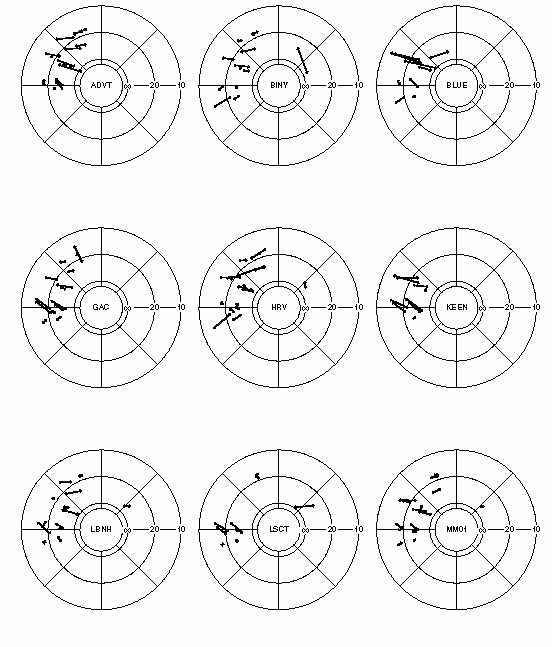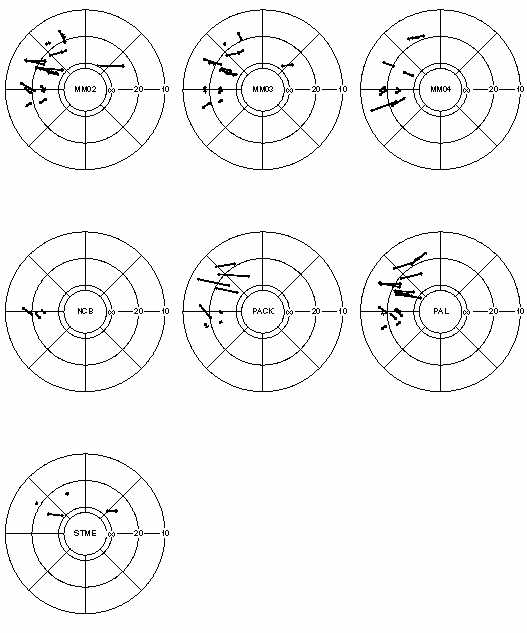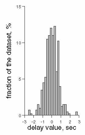
Figure 6. A histogram of relative traveltime delays determined for the network. The majority of delays do not exceed 1.5 s. (Postscript Version).

Figure 7. Relative delays determined for the stations of the network. Positive delays (crosses) and negative delays (triangles) are plotted as a function of backazimuth and phase velocity. (Postscript versions: Fig 7.1, Fig 7.2).

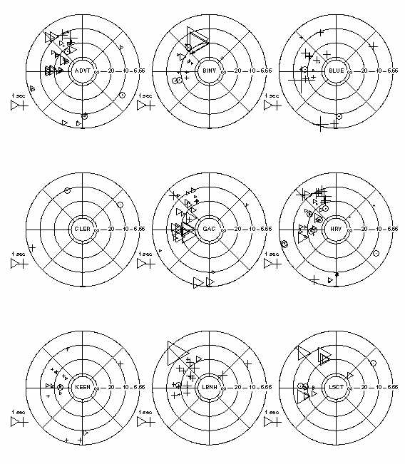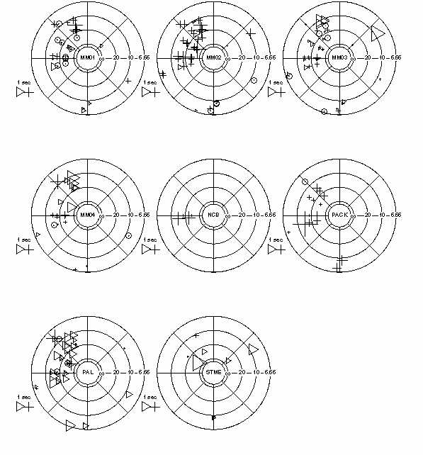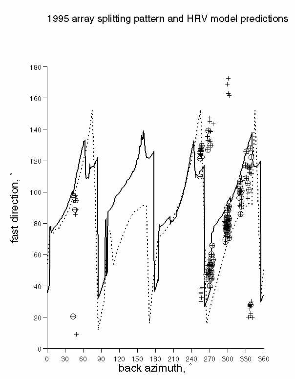
Figure 8. Variation of fast direction with backazimuth. All stations in the region appear to have the same pattern. Crosses show all measurements, circles identify measurements with . Predicted patterns of fast direction variation for two-layer models with hexagonal (dashed line) and orthorhombic (solid line) symmetries match the observations. The model was developed for station HRV [Levin et al., 1999], and is presented in Table 3. (Postscript Version).

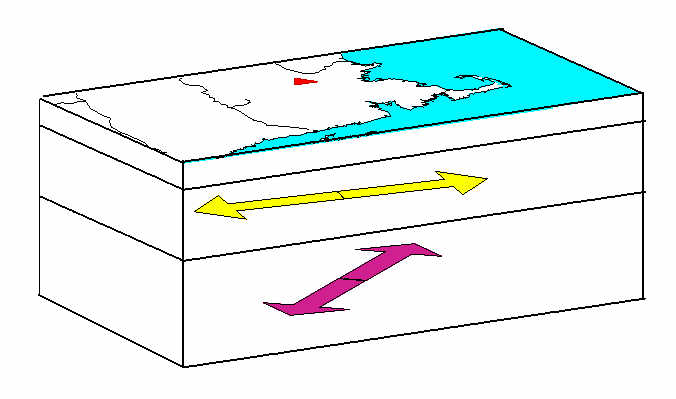
Figure 9. A schematic representation of the model for seismic anisotropy distribution under HRV. Station location is indicated by the triangle. See Table 3 for model parameters. (Postscript Version).

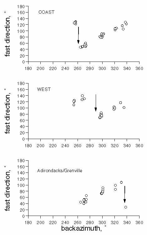
Figure 10. Regional variation in the pattern of fast direction change with backazimuth. Only high quality observations (circles from figure 9) are retained. (Postscript Version).

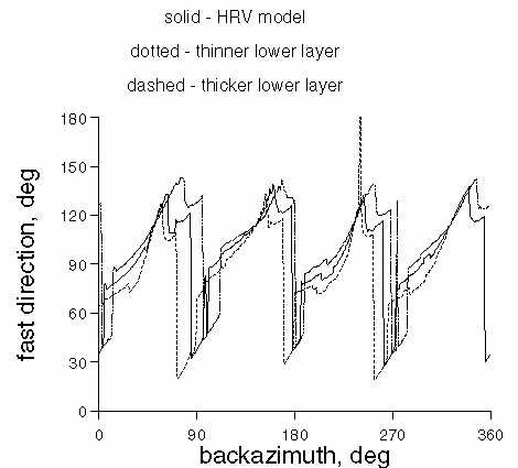
Figure 11. Changes in the pattern of fast direction change with backazimuth resulting from minor perturbations to the anisotropic model shown on Figure 9 and in Table 3. Thicknesses of two anisotropic layers in the HRV model (solid line) were perturbed by km, with the total thickness of the model being preserved. Dashed line shows a case of the thinner upper layer, dotted line - a thicker upper layer. The deviations of the pattern are comparable to those seen in the data. (Postscript Version).

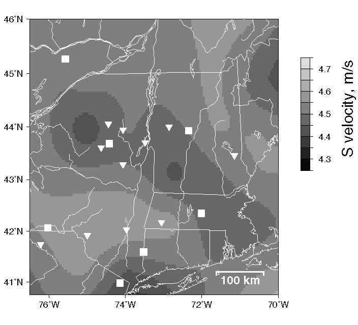
Figure 12. Distribution of shear velocity in the best-resolved region of the tomographic model (100 - 200 km deep). Velocity varies by , with lateral scale of anomalies being between 100 and 200 km. (Postscript Version).