THE ANTARCTIC DIPOLE

A Standing Wave in the Western Hemisphere of the Antarctic

What is the Antarctic Dipole (ADP)?

The Antarctic Dipole in Sea Ice Edge anomaly

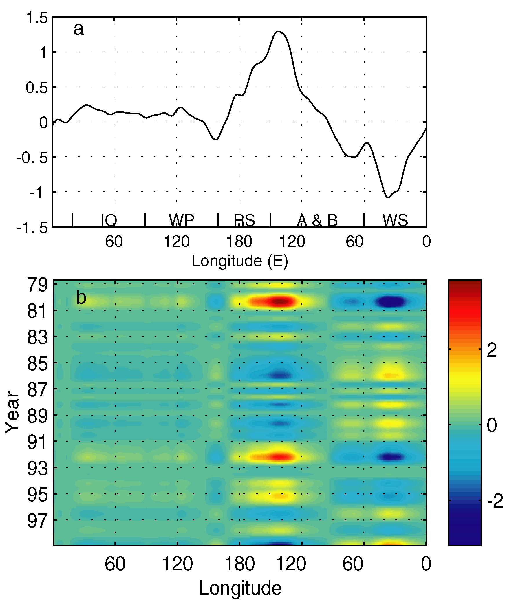
	The Antarctic Dipole best presents in the first EOF mode of sea ice edge anomalies (37% of total variance). The first eigenvector (a) has a peak in the western Amundsen Sea and a peak with opposite sign in the Weddell Sea. The reconstructed sea ice edge anomalies from the first mode (b) emphasizes the dipole's nature as a standing wave. The sea ice edge (30% of ice concentration) data were derived from monthly sea ice concentration generated by the bootstrap algorithm from NASA micorwave imagers from 10/1978 to 12/1999. The seasonal means were subtracted to yield anomaly field. The anomaly data were low-pass filtered to remove subannual variability before the EOF analysis.

The Antarctic Dipole in Surface Air Temperature anomaly

	The Antarctic Dipole best presents in the first two EOF modes of surface air temperature anomalies along 65S (53% of total variance). The combined eigenvector (c) and reconstracted temperature anomaly from these two modes (d) reveal the same dipole pattern. Surface air temperature was taken from NCEP/NCAR reanalysis air temperature at the 1000mb surface from 1/1975 to 12/1999 (plotted in the same period as sea ice data). The similar data processes had beed done as to the sea ice data.

The ADP and ACW

		Much of the interannual variability in the Southern Ocean has been described in the context of an Antarctic Circumpolar Wave (ACW) -- a wavenumber two phenomenon propagating in ice, pressure, wind and temperature fields around the Antarctic (White and Peterson, 1996). Here we compare the variance of the ADP (represented by the first two modes of sea ice and surface air temperature, and the third mode of sea level pressure, plotted in blue) and ACW (bandpass filtered between 3 and 7 years, plotted in red) with the total variance of the fields (plotted in green). The surface temperature and pressure data were taken from NCEP/NCAR reanalysis along 65S. Clearly, the ADP dominates variability in ice and temperature fields. The ADP and ACW are comparable in the pressure fields. Since the ACW and ADP have approximate the same wavelength and similar period, they are likely related. Likely relationships include: (1) The ACW propages through the area and excites the standing wave, and (2) the ADP is excited by extra-polar teleconnections and its anomaly is advected out of the dipole area by the Antarctic Circumpolar Current and/or air-sea-ice coupling processes. We favor the latter relationship for the following three reasons: (1) The eastern Pacific and Weddell Sea regions are very sensitive to extra-polar climate (Yuan and Martinson, 2000), (2) the ADP in sea ice can be predicted by extra-polar climate under certain conditions, and (3) the magnitude of ADP variability is much larger than the ACW.

Dipole's relationship with ENSO

The Teleconnection Pattern

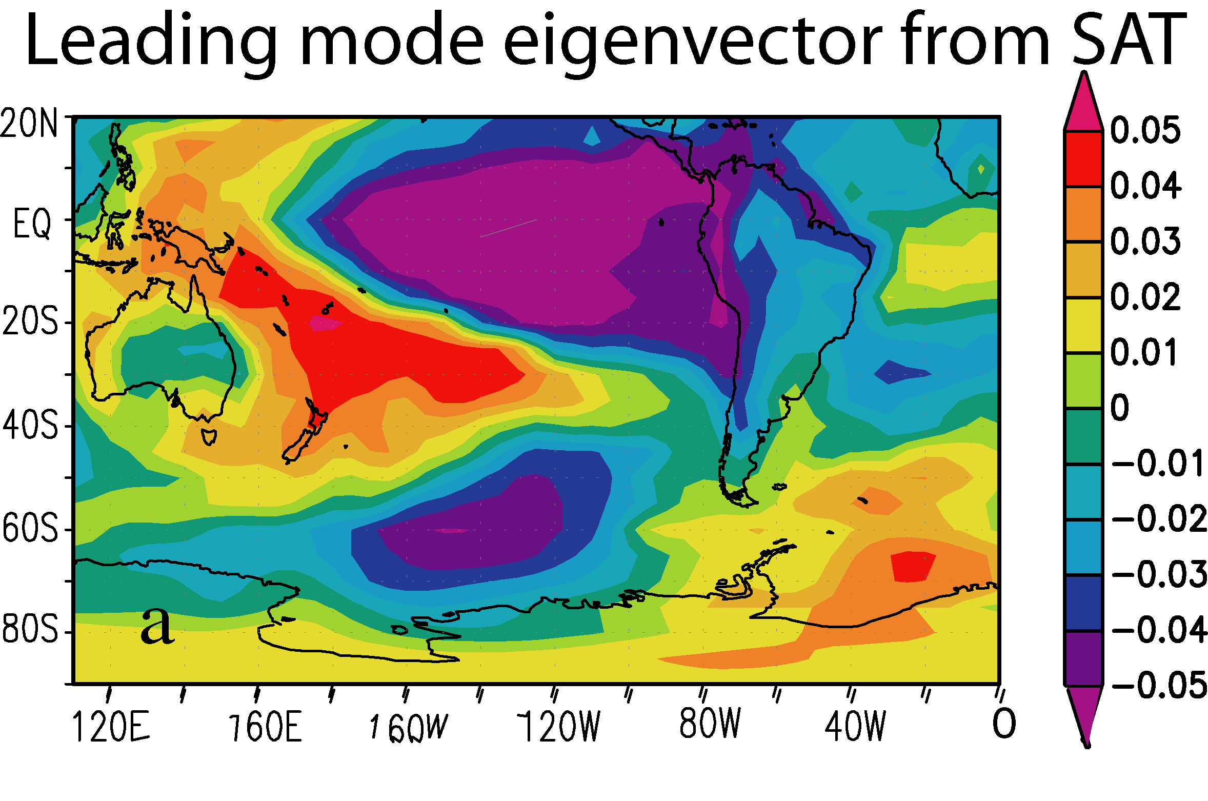		The leading mode of EOF analysis conducted on the surface air temperature anomaly in the Pacific and Atlantic south of 20N reveals a clear pattern linking the tropical Pacific and the dipole region in the Southern Ocean. The eigenvector shows a characteristic ENSO pattern with maximun amplitude in the central tropical Pacific. Associated with this ENSO pattern is a circumpolar pattern that resembles the Antarctic Dipole in the ice edge field, showing a pole in the near 60S in the South Pacific (of like-phase to the tropical signal) and another pole of opposite phase in the Weddell Sea.





Responses of Sea Ice Edge to ENSO Events

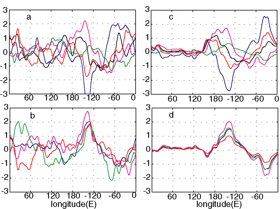		This figure shows September (the maximum ice coverage in the Southern Hemisphere) sea ice edge anomaly as function of longitude following five El Nino events in 1980, 1983, 1988, 1992 and 1997 (a) and four La Nina events in 1985, 1989, 1996 and 1999 (b). In the same way, September sea ice edge anomaly containing only the first EOF mode in the same El Nino years (c) and La Nina year (d). The ice edge anomaly in the dipole region responds to the tropical conditions much more regularly than the ice edge in other regions. Also apparent is the fact that the ice edge anomaly in the dipole regions responds more consistently to La Nina conditions than to El Nino conditions. The leading EOF mode strikingly domenstrates the later phenomenon.




The Spatial Scale of ENSO Influences

		The ENSO impact is generated by subtracting mean ice concetration at each month following La Nina events (above mentioned 4 years) from the mean ice concentration at each month following El Nino events (above mentioned 5 years). The white (black) line indicates the mean ice adge following El Nino events (La Nina events). The figure shows the ENSO impact in following September. The impact is stronger in the dipole regions than in other regions. Moreover, the impact is more or less limited near the ice edge. The ENSO influence on ice deep into the basins is rather small.




See the seasonal cycle of the ENSO Impact on ice pack in movies


See the paper