With the MB-System™ Format ID identified and the files copied to a manageable format, the next step is to take a look at the data. The things we want to accomplish are:
Organize the data set into a larger body of data you may already have.
Organize the data set internally, identifying specific areas that may require special processing.
Get a qualitative feel for the data to better understand what we are up against. Is the data generally free of errors or are there frequent outliers in the contours? Are there any longitudinal striations that might be caused by excessive ship noise? Do the outer beams exhibit depth excursions that might be indicative of large SSP errors? The idea is not to conduct an exhaustive examination, but to pick a few files through the data set to get a rough feel for how things look.
Extract the Latitude and Longitude as well as depth bounds of the data set. These values aid in future calculations and provide a framework for splitting up the processing of the data into chunks based on similar environmental conditions.
Evaluate the navigation information embedded in the data set. Is the navigation information smooth, or are there frequent outliers? Do data sets measured over the same area result in similar bathymetry, or are they offset due to navigation errors?
Often research institutions may maintain an single archive of several multibeam data sets from various cruises and various surveys. We might quickly consider how one might organize such an archive, to ease the task of processing and data retrieval.
Consider our example Lo'ihi data set. The top level directory of the Lo'ihi archive provided is entitled loihi. This is actually an unfortunate name on our part. Data sets should not be organized based on geographic location, as we shall explain. It might have been more appropriately entitled multibeam_archive. But for the time being we'll stick with loihi.
Organization below the top level directory can be quite varied, however should follow a single axiom - Data sets should not be organized by parameters that are easily managed by MB-System™. Two particular examples come to mind: time and space.
Managing data sets manually, by the time or location, is difficult, if not impossible to do. A common way to organize data sets is by cruise. (Alternatively, some institutions will organize data sets by principle investigator to allow administrative control over "ownership" and release of the data.) Cruises can be further broken down into segments, such that data is grouped in portions that require like processing or are simply in smaller chunks.
An example follows with segment directories shown for just one of the cruises.
archive/ewing_0101
archive/ewing_0101/segment_001
archive/ewing_0101/segment_002
archive/ewing_0101/segment_003
archive/ewing_0102
archive/ewing_0103
archive/knorr_0101
archive/knorr_0102
archive/knorr_0103
archive/knorr_0104
archive/thom_0101
archive/thom_0102
archive/thom_0103
The granularity of the file system within the archive will differ greatly from implementation to implementation, but the general idea is the same. With the hierarchy of directories and data files in place, we then create a series of recursive datalists within each directory.
Now consider our example data. Within our top archive directory, loihi we have subdirectories for each cruise. We might have broken these down further into segments if the data warranted, but in this case it did not. A diagram of the structure and a listing of the loihi directory are provided below.
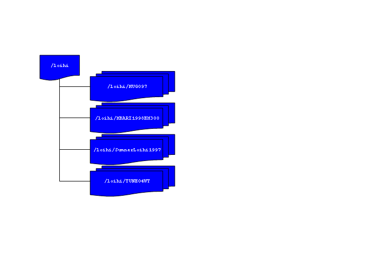
>ls -1 loihi
datalist.mb-1
datalistp.mb-1
HUGO97
MBARI1998EM300
SumnerLoihi1997
TUNE04WT
Note
For the moment disregard the file datalistp.mb-1. This data list will be used to specify that processed files are to take precedence over their unprocessed originals. The utility of this file will be covered in detail later on.
In the loihi directory we create the archive data list - datalist.mb-1. This file is a text file containing the relative path and name of each of the data lists in the successive lower level subdirectories. With each list file name is a special MB-System™ Format ID ("-1") denoting that formats will be specified in the lower recursed data lists. Also included a data weighting factor or "grid weight". The contents of datalist.mb-1 are shown below:
>cat datalist.mb-1
HUGO97/datalist.mb-1 -1 100.0
MBARI1998EM300/datalist.mb-1 -1 1.0
SumnerLoihi1997/datalist.mb-1 -1 0.1
TUNE04WT/datalist.mb-1 -1 0.001
Before we continue, consider the weighting factors above. The grid weighting factor is a way to merge multiple data sets over the same geographic area and prioritize which data will be extracted for display. Larger weighting factors take priority over smaller ones. While occasionally mitigating factors affect individual sonar performance, usually the difference in sonar quality between sonar vendor and even by vendor models are quite significant. Therefore, weighting data sets by "sonar model" is often a good practice. One might further refine the weighting factor by sonar model and ship, since differences in ship size and construction can significantly affect sonar data results. Increments between weights should be large to allow further refinement without added hassle. Toward that end, some organizations weight their datasets logarithmically as we have done here.
If we now consider the lower level data lists we see the format is similar, except now, instead of referring to lower level data lists, we refer directly to the data files themselves. For example, MBARI1998EM300/datalist.mb-1 contains a list of the data files and their format:
cat MBARI1998EM300/datalist.mb-1
mbari_1998_53_msn.mb57 57
mbari_1998_54_msn.mb57 57
mbari_1998_55_msn.mb57 57
mbari_1998_56_msn.mb57 57
mbari_1998_57_msn.mb57 57
mbari_1998_58_msn.mb57 57
mbari_1998_59_msn.mb57 57
mbari_1998_60_msn.mb57 57
mbari_1998_61_msn.mb57 57
Here no grid weight is included, although we could have specified one if a further level of granularity was required.
Note
The default behavior is for any grid weight in a particular datalist entry to override values derived from higher levels in the recursive structure. This behavior can be reversed if the text $NOLOCALWEIGHT is inserted in the data list (or in a datalist higher up in the structure).
In our Lo'ihi archive, we have only two layers of subdirectories, however we could have more. Recursive data lists would be created in a similar way, referring down through the structure until the actual data files are referenced. Typically upper level data lists are maintained manually, as they are small and easy to manipulate. However, in the lowest levels, creating a data list for a directory of hundreds of files can be cumbersome. mbdatalist can be used to generate these lists.
As an example, we'll create another data list for the MBARI1998EM300 data directory. First we need a text file with a list of the data files in the directory. To do that execute the following:
ls -1 | grep mb57 > list
We can then use this list with mbdatalist to create a data list as follows:
mbdatalist -F-1 -Ilist
mbari_1998_53_msn.mb57 57 1.000000
mbari_1998_54_msn.mb57 57 1.000000
mbari_1998_55_msn.mb57 57 1.000000
mbari_1998_56_msn.mb57 57 1.000000
mbari_1998_57_msn.mb57 57 1.000000
mbari_1998_58_msn.mb57 57 1.000000
mbari_1998_59_msn.mb57 57 1.000000
mbari_1998_60_msn.mb57 57 1.000000
mbari_1998_61_msn.mb57 57 1.000000
The results of the above command are sent to STDOUT, however the could have been redirected to a text file named datalist.mb-1 and we would essentially have the list we looked at earlier. We have now added a default grid weight of 1. Remember, the weights assigned here take precedence over those assigned higher in the recursion structure.
Note
Note that mbdatalist does not currently provide the ability to specify a weighting factor other than the default. It is primarily a data list parsing tool as we shall see in future examples. One can either manually specify the weight at a higher level in the data list recursion structure, or adjust the default grid weight via a simple shell script. The following example changes the default value to 100.
cat datalist_old | sed 's/1\.000000/100/' > datalist_new
Finally we should remove our interim list
rm list
So what is the benefit of having our data in this archive, with all these recursive data lists?
Suppose you were interested in the highest quality data you have covering Lo'ihi and the surrounding area. You can now quickly make a mosaic of the various data sets, simply by referring to the archive data list rather than sorting through a myriad of data files to decide the best quality data to then refer to the files directly. Where two data sets are collocated, the data with the highest grid weight will be extracted.
As we continue with data processing, we'll create post-processed data files adjacent to the raw data files in the archive. mbdatalist allows us to insert a flag ("$PROCESSED") into any data list causing the processed versions of the data in that list, and those beneath it in the recursion structure, to be extracted rather than the raw, unprocessed data. In this way we may selectively extract the processed or non-processed data files within our data structure. As an illustration, you'll find a secondary data list in the highest level directory called datalistp.mb-1 which contains only two entries - the $PROCESSED flag and the original archive data list datalist.mb-1.
Note
Alternatively, mbdatalist can be called with the -P flag which sets the $PROCESSED flag and overrides all others.
Similar to the discussion above, a "$RAW" flag in a data list or the -U flag on the command line can be specified to explicitly extract only the unprocessed data files, either by data list or universally as above.
Suppose we want to know the geographic bounds of the entire Lo'ihi archive. We simply run mbinfo and refer to the highest level data list to get statistics regarding the entire archive.
 mbinfo -F-1 -I datalist.mb-1
...

Data Totals:
Number of Records:           191764
Bathymetry Data (135 beams):
  Number of Beams:         12119082
  Number of Good Beams:     8745488     72.16%
  Number of Zero Beams:     1590395     13.12%
  Number of Flagged Beams:  1783199     14.71%
Amplitude Data (135 beams):
  Number of Beams:          7285751
  Number of Good Beams:     5519648     75.76%
  Number of Zero Beams:      608084      8.35%
  Number of Flagged Beams:  1158019     15.89%
Sidescan Data (1024 pixels):
  Number of Pixels:        10155008
  Number of Good Pixels:    4023419     39.62%
  Number of Zero Pixels:    6131589     60.38%
  Number of Flagged Pixels:       0      0.00%

Navigation Totals:
Total Time:         -49797.0534 hours
Total Track Length: 36092.8118 km
Average Speed:          0.0000 km/hr ( 0.0000 knots)

Start of Data:
Time:  06 21 1997 19:01:07.393000  JD172
Lon: -155.2214     Lat:   18.8823     Depth:   301.0800 meters
Speed:  1.9631 km/hr ( 1.0611 knots)  Heading: 229.1400 degrees
Sonar Depth:    0.3000 m  Sonar Altitude:  300.7800 m

End of Data:
Time:  10 16 1991 21:57:55.000000  JD289
Lon: -157.8782     Lat:   21.2853     Depth:    33.0000 meters
Speed: 20.5175 km/hr (11.0906 knots)  Heading:  31.2014 degrees
Sonar Depth:    0.0000 m  Sonar Altitude:   33.0000 m

Limits:
Minimum Longitude:    -157.8801   Maximum Longitude:    -153.3829
Minimum Latitude:       18.5684   Maximum Latitude:       21.2853
Minimum Sonar Depth:    -0.4100   Maximum Sonar Depth:  1530.3800
Minimum Altitude:      -92.9500   Maximum Altitude:     5482.8000
Minimum Depth:          33.0000   Maximum Depth:        5605.0000
Minimum Amplitude:     -60.0000   Maximum Amplitude:     255.0000
Minimum Sidescan:        0.1600   Maximum Sidescan:       90.5000
In these results we see that information regarding track length, speed, and duration are incorrect. mbinfo as they become meaningless when considering multiple overlapping data sets taken on different ships at different times. However the geographic and depth "Limits" are reported correctly as are the beam statistics. For example, here we see the archive has a minimum depth of 33 meters and maximum depth of 5604 meters.
Suppose you are interested in which data files contain data covering the top of Lo'ihi. We can use mbdatalist to create an extraction data list that covers only data files containing data within specified geographic bounds, for example:
mbdatalist -F-1 -I datalist.mb-1 -R-155.5/-155/18.7/19.2
results in the following data list containing with data within the bounds -155.5/-155/18.7/19.2. :
HUGO97/mba97172L05.mb121 121 100.000000
HUGO97/mba97174L01.mb121 121 100.000000
HUGO97/mba97174L02.mb121 121 100.000000
HUGO97/mba97174L04.mb121 121 100.000000
HUGO97/mba97174L05.mb121 121 100.000000
HUGO97/mba97174L06.mb121 121 100.000000
HUGO97/mba97174L07.mb121 121 100.000000
HUGO97/mba97175L01.mb121 121 100.000000
HUGO97/mba97175L03.mb121 121 100.000000
MBARI1998EM300/mbari_1998_53_msn.mb57 57 1.000000
MBARI1998EM300/mbari_1998_54_msn.mb57 57 1.000000
MBARI1998EM300/mbari_1998_55_msn.mb57 57 1.000000
MBARI1998EM300/mbari_1998_56_msn.mb57 57 1.000000
MBARI1998EM300/mbari_1998_57_msn.mb57 57 1.000000
MBARI1998EM300/mbari_1998_58_msn.mb57 57 1.000000
MBARI1998EM300/mbari_1998_59_msn.mb57 57 1.000000
MBARI1998EM300/mbari_1998_60_msn.mb57 57 1.000000
MBARI1998EM300/mbari_1998_61_msn.mb57 57 1.000000
SumnerLoihi1997/61mba97043.d01 121 0.100000
SumnerLoihi1997/61mba97043.d02 121 0.100000
SumnerLoihi1997/61mba97044.d01 121 0.100000
SumnerLoihi1997/61mba97044.d02 121 0.100000
TUNE04WT/TUNE04WT.SWSB.91oct08 16 0.001000
TUNE04WT/TUNE04WT.SWSB.91oct09 16 0.001000
TUNE04WT/TUNE04WT.SWSB.91oct10 16 0.001000
TUNE04WT/TUNE04WT.SWSB.91oct11 16 0.001000
At the time of this writing, mbcopy does not support the datalist feature. However, we can write a simple script to extract the files in our data list to the local directory. As an example, a quick script is included here:
#!/usr/bin/perl
#
# Program Name: archiveExt
#
# Usage: cat datalist | ./archiveExt
#
# Val Schmidt
# Lamont Doherty Earth Observatory
#
#
# This script takes a datalist of files in an archive
# and extracts a copy of them to the local directory.
# No change in format is applied, however that is easily modified.
# Files not using the standard MB-System suffix (mb###) will have
# one appended.

while (<>){
        ($file,$format,$gridweight)=split(" ",$_);
        $infile=$file;
        # look for standard suffix and remove it if it exists
        if (($file=~m/mb...$/) || ($file=~m/mb..$/)){
                $file=~s/\.mb.*//;      # remove suffix
        }
        $file=~s/^.*\///g;      # remove leading path
        $outfile=$file;
        $cmd="mbcopy -F$format/$format -I$infile"." -O".$outfile."\.mb"."$format";
#           print "$cmd\n";
            system($cmd);

    }
With the data files extracted from the archive we can write them to some portable media and port them where ever we like.
As you can see data archives with systematic recursive data lists, combined with the MB-System™ tool mbdatalist provide a powerful tool for managing your data set within a larger archive.
Now that our MBARI1998EM300 data set has a home within our larger archive, we turn to looking at the data itself to determine if there is a need to further segment the data - "Divide and Conquer!" In general, it is usually helpful to segment the data into portions that require unique processing. One might place each subset into its own directory with its own recursive data list. This is a good time to take a close look at the notes that you have painstakingly taken during the cruise. They can be invaluable in providing clues for portions of the data that might be troublesome. This is also where you typically curse yourself, or someone else, for a lack of detail.
For example, suppose on the 31st day of a 45 day cruise, the ship's heading reference fails. Six hours later, a marine tech has suspended a magnetic needle from a string. And with a laser diode from a CD player a reflector, and a series of photo-transistors managed to restore the ship's heading to the sonar system. While far from perfect, the sonar has a modest idea of the ship's heading. But where before the multibeam data looked as though you'd painted the sea floor with a roller, it now looks like a Jackson Pollack painting. Post processing this data is not impossible, but certainly different than the typical multibeam data set and should be conducted separately from the rest of the data.
Or more simply, suppose your mapping near the edge of the Gulf Stream, and you've seen from the many XBT's shot during the cruise that there was a somewhat dramatic change in sound speed profile across what you suspect was a large eddy. Since you expect to be applying different sound speed profiles to each subset of the data, you might decide to segment the data around this change in sound speed profile.
Caution
When participating in a cruise it is imperative to consider in advance the kinds of things that could go wrong in a multibeam data set. Train watchstanders to look for and log changes in sound speed profile, operation of the ship's heading and attitude reference, GPS receiver operation, changes in sea state, and MOST IMPORTANTLY operation of the temperature instruments that provide the speed of sound at the keel. This final factor is the one element that cannot be corrected in post processing. Good notes provide lots of clues regarding how to fix data sets and provide immeasurable peace of mind when you find yourself presenting your data before your peers.
Clearly segmenting the data is something of an iterative process. As you look more closely at your data set and get further into the post processing, you may rearrange you plan of attack and change your organization structure. One must not get frustrated, but simply sigh and understand that it is part and parcel of the process.
Before we continue, it seems as good a time as any to describe the various ancillary data files generated and used by MB-System™. After a brief introduction to them we'll generate a few standard ones for our data set automatically with mbdatalist.
The ancillary data files provide statistics, metadata and abbreviated data formats for the manipulation, display and post processing of the multibeam data. A summary description for each is provided below.
.inf - file statistics
These files contain metadata about the multibeam data, including geographic, temporal and depth bounds, ship track information, and numbers of flagged or zero beams. They are created by mbinfo, often via mbdatalist and automatically via mbprocess.
.fbt - fast bathymetry
These files are bathymetry only format 71 files that are intended to provide faster access to swath bathymetry data than in the original format. These are created only for data formats that are slow to read. These are generated using mbcopy typically via mbdatalist or automatically through mbprocess.
.fnv - fast navigation
These files are simply ASCII navigation files that are intended to provide faster access to swath navigation than data in the original format. These are created for all swath data formats except single beam, navigation, XYZ. These are generated using mblist, typically via mbdatalist and automatically by mbprocess.
.par - parameter files
These files specify settings and parameters controlling how mbprocess generates a processed swath data file from a raw swath data file. These are generated or updated by all of the data editing and analysis tools, including mbedit, mbnavedit, mbvelocitytool, mbclean, mbbackangle, and mbnavadjust. They are also directly altered by mbset.
.esf - bathymetry edit flags
These files contain the bathymetry edit flags output by mbedit and/or mbclean.
.nve - edited navigation
These files contain the edited navigation output by mbnavedit.
.na0, .na1, .na2, .na3 ... - edited navigation
These files contain adjusted navigation output by mbnavadjust. These navigation files generally supersede .nve files output by mbnavedit. The latest (highest number) .nv# files are used so .na2 will supersede na1.
.svp - sound velocity profile
These files contain a sound velocity profile used in recalculating bathymetry. The .svp files may derive from mblevitus, mbvelocitytool, mbm_xbt, or other sources.
We can now use mbdatalist to generate, for each data file, summary statistics and special bathymetry and navigation data that is more easily read by MB-System™ tools. This excerpt from the mbdatalist man page is helpful in understanding how they fit into the big picture:
MB-System™ makes use of ancillary data files in a number of instances. The most prominent ancillary files are metadata or "inf" files (created from the output of mbinfo). Programs such as mbgrid and mbm_plot try to check "inf" files to see if the corresponding data files include data within desired areas. Additional ancillary files are used to speed plotting and gridding functions. The "fast bath" or "fbt" files are generated by copying the swath bathymetry to a sparse, quickly read format (format 71). The "fast nav" or "fnv" files are just ASCII lists of navigation generated using mblist with a -OtMXYHSc option. Programs such as mbgrid, mbswath, and mbcontour will try to read "fbt" and "fnv" files instead of the full data files whenever only bathymetry or navigation information are required.
To generate these ancillary data files, from within the MBARI1998EM300 directory, we execute mbdatalist with the -N flag:
mbdatalist -F-1 -I datalist.mb-1 -N
Now the directory looks like the following:
ls
datalist.mb-1               mbari_1998_57_msn.mb57.fnv
mbari_1998_53_msn.mb57      mbari_1998_57_msn.mb57.inf
mbari_1998_53_msn.mb57.fbt  mbari_1998_58_msn.mb57
mbari_1998_53_msn.mb57.fnv  mbari_1998_58_msn.mb57.fbt
mbari_1998_53_msn.mb57.inf  mbari_1998_58_msn.mb57.fnv
mbari_1998_54_msn.mb57      mbari_1998_58_msn.mb57.inf
mbari_1998_54_msn.mb57.fbt  mbari_1998_59_msn.mb57
mbari_1998_54_msn.mb57.fnv  mbari_1998_59_msn.mb57.fbt
mbari_1998_54_msn.mb57.inf  mbari_1998_59_msn.mb57.fnv
mbari_1998_55_msn.mb57      mbari_1998_59_msn.mb57.inf
mbari_1998_55_msn.mb57.fbt  mbari_1998_60_msn.mb57
mbari_1998_55_msn.mb57.fnv  mbari_1998_60_msn.mb57.fbt
mbari_1998_55_msn.mb57.inf  mbari_1998_60_msn.mb57.fnv
mbari_1998_56_msn.mb57      mbari_1998_60_msn.mb57.inf
mbari_1998_56_msn.mb57.fbt  mbari_1998_61_msn.mb57
mbari_1998_56_msn.mb57.fnv  mbari_1998_61_msn.mb57.fbt
mbari_1998_56_msn.mb57.inf  mbari_1998_61_msn.mb57.fnv
mbari_1998_57_msn.mb57      mbari_1998_61_msn.mb57.inf
Each of the tree types of data ancillary data files have been created for each data file in the original directory. This is a good time to create ancillary data files for all the data you will be processing as they will be greatly speed the process.
Now we need to take a quick look at our data and get a feel for what we're up against. This is much the same process described in the "Surveying your Survey" chapter. The idea is to get an idea of its quality and the lay of the sea floor.
First lets generate a navigation plot:
mbm_plot -F-1 -I datalist.mb-1 -N
And here's the resulting plot:
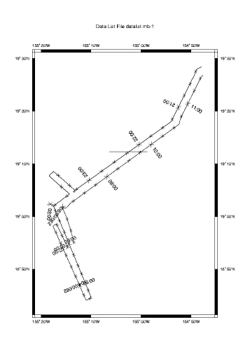
Here we can see the ship's track coming in from the North East, a small mapping pattern over the summit of Lo'ihi and the return trip.
We can also see what appears to be an extraneous line on the plot at roughly 19'12"N. We note this irregularity as something to investigate.
If we look close there appears to be discontinuities along the ship's track at roughly 19'02"N 155'16W (0200) and 18'55"N 155'15"W (0700). So we look focus a our plot a bit, using the -R flag to specify geographic bounds to mbm_plot, and look again.
mbm_plot -F-1 -I datalist.mb-1 -N -R-155.33/-155.14/18.7/19.15
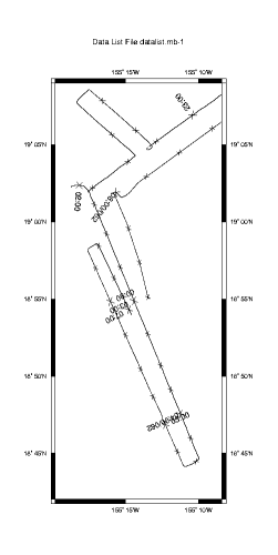
We clearly see two discontinuities in the navigation data. Have we lost our navigation source? Was there a problem with the sonar? Is there a portion of the data set missing? Anyone who has spend much time processing multibeam data has spent multitudes of time trying to answer these kinds of questions, however, it shouldn't be a process of data forensics. The answer should be in the cruise notes - a lesson that cannot be stressed enough.
In this case the answer is "none of the above". The notes say that this data set was taken by a commercial survey outfit. Commercial ships tend to only take data when they are absolutely required. Therefore, they frequently secure their data systems when outside the contracted survey area, or during turns, when a poor ship's vertical reference will make the data all but unusable. The "missing" data segments shown in the plot are a result and we know this because we took good notes during the cruise. Good notes are essential to post processing.
Note
The practice of securing sonars during turns often seems stingy to most scientists, who prefer to err on the side of collecting all the data they can. This comes with a price however. Considerable amounts of time and money are often then required to flag beams during turns or other events that prevent the taking of usable data.
Now we should take a look at a contour plot, as it can give us a better idea of the noise in the data set. Here we look primarily for contours that are jagged and irregular to signify data that requires editing.
mbm_plot -F-1 -I datalist.mb-1 -C -G1
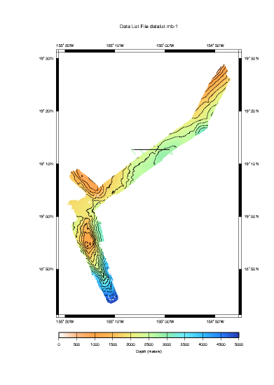
In the plot above we see that, in general, things look pretty good with two exceptions. The large line at 19'N is still apparent and appears to be more than a plotting artifact. Bathymetry data have been associated with the discontinuity placing small colored lines on our plot well outside our track and expected coverage. The deep water bathymetry at the bottom of the plot is also troublesome. Multibeam sonars radiate a fan shape from the bottom of the vessel, hence we expect the bathymetry map to widen with increasing water depth. Here however, the swath width narrows in a non-uniform way and data is lost near the center beam. These effects can be caused by a sonar that is not appropriately adjusting its power and gain settings dynamically with depth. Or perhaps something else is afoot. At any rate, it will no doubt require careful consideration.
We won't segment this small data set any further, however it is useful to know the bounds in time and space of the entire data set so we run mbinfo
mbinfo -F-1 -I MBARI1998EM300/datalist.mb-1
... and the results:
Data Totals:
Number of Records:             9917
Bathymetry Data (135 beams):
  Number of Beams:          1338795
  Number of Good Beams:     1207888     90.22%
  Number of Zero Beams:       79143      5.91%
  Number of Flagged Beams:    51764      3.87%
Amplitude Data (135 beams):
  Number of Beams:          1338795
  Number of Good Beams:     1207888     90.22%
  Number of Zero Beams:       79143      5.91%
  Number of Flagged Beams:    51764      3.87%
Sidescan Data (1024 pixels):
  Number of Pixels:        10155008
  Number of Good Pixels:    4023419     39.62%
  Number of Zero Pixels:    6131589     60.38%
  Number of Flagged Pixels:       0      0.00%

Navigation Totals:
Total Time:            15.4770 hours
Total Track Length:   286.9084 km
Average Speed:         18.5377 km/hr (10.0204 knots)

Start of Data:
Time:  03 02 1998 20:06:01.740000  JD61
Lon: -154.7988     Lat:   19.4734     Depth:  1000.6700 meters
Speed: 18.0000 km/hr ( 9.7297 knots)  Heading: 243.2100 degrees
Sonar Depth:    6.0700 m  Sonar Altitude:  988.5300 m

End of Data:
Time:  03 03 1998 11:34:38.985000  JD62
Lon: -154.7938     Lat:   19.4458     Depth:  1502.0900 meters
Speed: 18.0000 km/hr ( 9.7297 knots)  Heading:  59.4300 degrees
Sonar Depth:    5.0100 m  Sonar Altitude: 1492.0700 m

Limits:
Minimum Longitude:    -155.3265   Maximum Longitude:    -154.7814
Minimum Latitude:       18.7261   Maximum Latitude:       19.4817
Minimum Sonar Depth:     3.8700   Maximum Sonar Depth:     7.4600
Minimum Altitude:      695.0300   Maximum Altitude:     4861.8900
Minimum Depth:         331.8400   Maximum Depth:        4919.0700
Minimum Amplitude:       2.0000   Maximum Amplitude:      58.5000
Minimum Sidescan:        0.1600   Maximum Sidescan:       90.5000
Gaining some knowledge about our data set and its potential problems is just the first step in preparing to process the data. Before we can conduct our final processing we need to eliminate other errors. Among these are the ship and sonars roll and pitch biases. So we move on to that topic next.