When a ship is at sea, the sonar array is continuously moving with respect to the sea floor due to the ship's motion. The sonar must then continuously correct the sonar data for the ship's motion by comparing the orientation of the ship at any instance with some some known vertical reference. Most sonars take input from separate gyroscopic or inertial navigation systems which provide these corrections in real time.
Roll bias is a measure of the difference between the athwartships alignment of the ship's multibeam hydrophone array, and that of its vertical reference source. Although the installation of both the hydrophone array and the inertial navigation system are done with the utmost care to minimize these differences, some error always exists. Moreover, over the course of the life of a ship the values will change and should be periodically remeasured.
Note
Roll bias is frequently misunderstood to be a measure of the difference between the sonars alignment and the true vertical. This is not the case, and can cause considerable confusion when troubleshooting and trying to understand abnormal tilts in a data set. The measurement of roll bias, as we shall see, is between the ships vertical reference and the sonar. The assumption is made that errors in the ships vertical reference from the true vertical average out over time such that the reference approximates the true vertical, however this is not always the case.
A correction to the current roll bias value is measured by taking two sets of data over a planar bottom while sailing nearly exact reciprocal courses. (Note that the sea floor need not be level, but must be as planar as possible, ideally with any slope perpendicular to the course of the ship.) The two data sets are then fit to planes and an angular athwartships deviation is calculated between them. This value is then applied as a correction to the current roll bias in the system.
The example that follows is a narrative discussion of a roll bias calculation performed aboard the R/V Ewing in the spring of 2002.
Data was taken for the roll bias calculations during the transit between Guam and Dutch Harbor, Alaska. A possible flat bottom area was found by chart review. During the transit over this area, the Hydrosweep was carefully watched to find the a stretch of planar sea floor suitable to conduct the test.
The ship was in water of about 5700 meters. This translated into a ping interval of about 20 sec. We therefore decided on a data set 45 min long in each direction to give us some 150 ping returns. To reduce the ship's noise in the data set we slowed to 8 knots during the runs.
After identifying a good 45 min stretch of sea floor we noted it's beginning latitude and longitude and went to the bridge. We asked the helm to mark our current position, conduct a Williamson turn and slow to 8 knots, retrace our track to our beginning point, conduct a second Williamson to resume base course, and finally notify us when they had reached the starting point, after which they could resume their transit speed.
Our resulting data files covered 200204282310 - 20020429010010 GMT.
The Data Manipulation strategy is to convert the "raw" data files to a more manageable format, plot the data such that exact start and stop times can be identified for each course, and finally extract data for each track using these start and stop times to create composite data files for each reciprocal course track. These composite data files can then be directly input into the MB-System™ mbrollbias process.
The raw data files, retrieved directly from the sonar workstation, each contain 10 minutes of data and are in the "182" MB-System™ format.
A 10 minute file set in the "182" format contains 9 files. While the bathymetry is primarily contained in the .fsw files the remaining 8 files are also required.
Once copied to a working directory the files were converted to a more manageable 183 format using mbcopy. A small script was written to do them all in one step.
#!/usr/bin/perl
#
#
# Usage: ls -1 | ./multi-copy
#
# Val Schmidt
# Lamont Doherty Earth Observatory
#
# This script takes a directory full to 182 format multi
# beam files and converts them to 183 format files.

while (< >){
        if (/.*fsw$/){
            chomp;
            s/$_/\.fsw$//;
            $cmd="mbcopy -F182/183 -I$_"."\.fsw"." -O"."$_"."\.mb183";
            #print $cmd;
            system($cmd);
        }
    }
Note
Subsequent beta versions of MB-System™ (5b29 and later) have included the new process mbm_copy which allows one to copy large numbers of data files between formats and obsoletes the need for this script. See, feedback works!
MB-System™ 's 183 format is compact, with only a single file for the bathymetry, navigation and other information. The results of the above script are single data files with the ".mb183" suffix appended to the end of their root filename. This suffix is recognized by MB-System™ interactive utilities such as mbedit and mbvelocitytool.
Times annotated in our notes during the rollbias data taking runs allowed us identify the files containing the bathymetry data for each track. A text file containing a list of these files and their format was created to facilitate the subsequent steps as shown below.
[vschmidt@val-ldeo rollbias]$ cat firsttrackformat
00020428232010.mb183 183
00020428233010.mb183 183
00020428234010.mb183 183
00020428235010.mb183 183
00020429000010.mb183 183
[vschmidt@val-ldeo rollbias]$ cat secondtrackformat
00020429001010.mb183 183
00020429002010.mb183 183
00020429003010.mb183 183
00020429004010.mb183 183
00020429005010.mb183 183
00020429010010.mb183 183
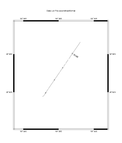
These data sets were then plotted to ensure they cover the reciprocal tracks and do not contain any extraneous data particularly the turns at the end of each leg.
mbm_plot -F-1 -I firsttrackformat
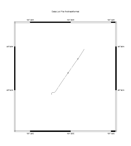
mbm_plot -F-1 -I secondtrackformat
As luck would have it, our first track contains a portion of the turn. We therefore have to window the data file to remove the unwanted section. The last data file in the first track list was the one that required windowing. By noting the time at which the turn started, a copy of the straight portion of the track could be extracted using mbcopy.
mbcopy -F183/183 -Iinputfilename -Ooutputfilename -BYYYY/MM/DD/HH/MM/SS -EYYYY/MM/DD/HH/MM/SS
We then augmented our "firsttrack" file list as shown below.
vschmidt@grampus:~/ewing/data/cruises/ew0204/rollbias% less firsttrack
00020428232010.mb183
00020428233010.mb183
00020428234010.mb183
00020428235010.mb183
00020429000010.copy.mb183
The mbrollbias process requires a single set in input files for each leg of the track. Armed with the firsttrack and secondtrack file list we created single composite data files for each track with the following lines shown below
cat firsttrack | xargs cat >> compositefirsttrack.mb183

cat firsttrack | xargs cat >> compositesecondtrack.mb183
Note
The concatenation of data files as shown below does not typically work with the "native" sonar formats.
So now we'd looked at the data from each track, windowed them appropriately to ensure we had exactly the data we wanted, and concatenated the data into single composite data files for each of the two reciprocal courses.
Now that we have extracted the data files, we needed to clean them up a bit. This was a straight forward manual process of running mbedit. From within mbedit we loaded the first data file.
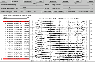
We used the Filters... selection under the Control button to flag the outer 10 beams on either side, as they are typically quite noisy. Then after adjusting the vertical scaling to something around 3 and increasing the number of beams displayed in each screen to something around 30, we carefully stepped through the entire data set. Using the "toggle" setting and mouse we flagged individual unruly or inconsistent beams. Occasionally an entire ping would be removed by first flagging a single beam and then typing z. When complete with the first file we clicked Quit which closed mbedit and saved a .par file for later processing of the flagged beams. The editing process was repeated for the second composite data file.
With the flagging of poor data complete for both data sets we ran mbprocess to apply the corrections and create new edited data sets.
mbprocess -Icompositefirsttrack.mb183 -F183
mbprocess -Icompositesecondtrack.mb183 -F183
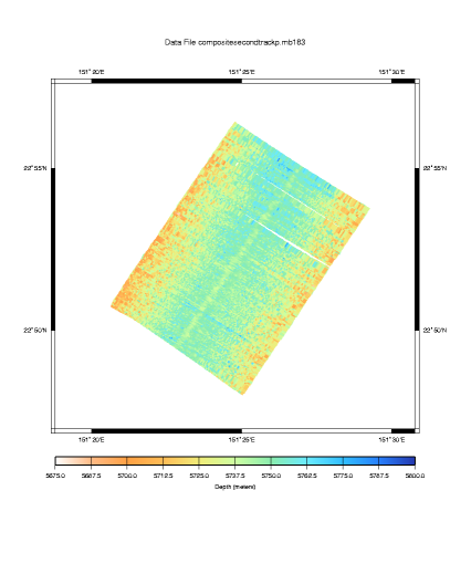
These lines result in processed data files named compositefirsttrackp.mb183 and compositesecondtrackp.mb183 respectively. For illustration they are plotted below.
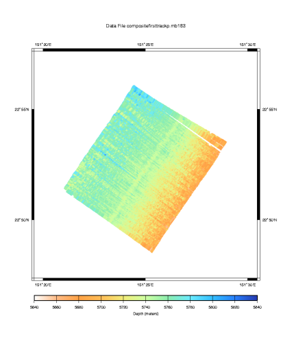
With nice clean data sets for each reciprocal track the set remaining is use mbrollbiasto conduct the final calculations. mbrollbias takes as arguments, the two input data file and their formats, as well as a region in latitude and longitude over which to calculate. mbrollbias splits this region into a grid and calculates roll bias values for each region. The number of grid squares can be specified with the -Dx/y argument. This can be helpful when the data only covers some small swath of a larger region. Alternatively mbrollbias can be forced to conduct the calculations over the composite whole returning only a single value using -D1/1. This is what we have done, our results are below.
mbrollbias -F183/183 -I compositefirsttrackp.mb183 \
-J compositesecondtrackp.mb183 -D1/1 -R151.4997/151/3344/22.7970/22.9520

MBROLLBIAS Parameters:
Input file 1:     compositefirsttrackp.mb183
Input file 2:     compositesecondtrackp.mb183
Region grid bounds:
  Longitude:  151.3344  151.4997
  Latitude:    22.7970   22.9520
Region grid dimensions: 1 1
Longitude interval: 0.165300 degrees or 16.962596 km
Latitude interval:  0.155000 degrees or 17.165048 km
Longitude flipping:   0

17902 depth points counted in compositefirsttrackp.mb183
19747 depth points counted in compositesecondtrackp.mb183
17902 depth points read from compositefirsttrackp.mb183
19747 depth points read from compositesecondtrackp.mb183

Region 0 (0 0) bounds:
    Longitude:  151.3344  151.4997
    Latitude:    22.7970   22.9520
First data file:    compositefirsttrackp.mb183
    Number of data: 17902
    Mean heading:   217.036742
    Plane fit:      5.750465 -0.006331 0.005092
Second data file:   compositesecondtrackp.mb183
    Number of data: 19747
    Mean heading:   31.696466
    Plane fit:      5.735079 0.000629 0.000129
Roll bias:   0.004220 (0.241800 degrees)
Roll bias is positive to starboard, negative to port.
A positive roll bias means the vertical reference used by
    the swath system is biased to starboard,
    giving rise to shallow bathymetry to port and
    deep bathymetry to starboard.
With the roll bias correction calculations complete, one may either set MB-System™ to apply these corrections to the data, or preferentially, the correction is entered into the multibeam sonar system such that corrections are made on the fly. Let us first look at how to apply the roll bias to the sonar data in post processing using MB-System™, as entering the value into the sonar sounds easy, but this process is sufficiently confusing it is well worth belaboring the details.
Applying roll bias corrections to sonar data only requires that we specify, in the ancillary parameter file (".par"), the roll bias to apply. This is done most easily using mbset. The syntax for such a statement might look like the following:
mbset -Idatalist-1 -PROLLBIASMODE:1 -PROLLBIAS:rollbias_value
In the line above, all the data files listed in datalist-1 will be affected. Parameters to be set are specified with the "-P" flag to mbset. A rollbias mode of 1 specifies that roll bias corrections should be processed, and that they should be applied to both the port and starboard beams equally. (Alternatively roll bias correction processing can be turned off - Mode 0, or applied with different biases for port and starboard beams - Mode 2) Finally, the roll bias value to apply is specified in the last argument. With the line above executed, subsequent execution of mbprocess will apply the roll bias corrections to that data.
Now we can move on to the delecate process of entering roll bias values directly into the sonar, such that the data is correct "right out of the box". The details of this should be routine to any ship with a multibeam sonar, and asking the right questions from knowledgeable people should illicit the correct answers. However often that is not the case, so an in depth discussion is worth while, in the event one has to figure it out on their own.
First one must know the polarity convention the sonar uses for roll - is a roll to STBD a positive value, or a negative one? Most sonars consider a roll to STBD as positive, but many have the ability to change this polarity convention via software or dip switch settings, so you'll have to investigate. It is typically not sufficient to look at the convention of the vertical reference. Vertical reference inputs often have user-selectable polarity for roll values as well. So while the sonar may think of a roll to STBD as positive, it may actually take a negative input for a STBD roll from the vertical reference. The true-blue test is to fake the roll value entered into the sonar and watch the cross track profile of the sonar swath. Many newer inertial navigation units have the ability to do just that. A simulated roll to port will have the effect of slanting the cross track profile down to STBD.
Next one must understand how the sonar applies the roll bias settings. For example, does the sonar's interface have the operator enter the sonar's measured roll bias value, which it then applies as a correction to (subtracts from) the real time roll, or does it have one enter the value as a the roll bias correction which it then simply applies (adds to) the real time roll. Unfortunately, sonar operator manuals often do not make these essential details clear, and one has to experiment with large values, inspect the sonar data, and convince yourself that you've got it right.
The final hurdle, is to understand that the value provided by mbrollbias is the actual roll bias as measured from the current settings in the sonar. If one were to "zero" the roll bias settings before collecting the data, the values provided by mbrollbias would be the absolute roll bias. However since we did not, in this example, the values provided are adjustments to the current values. That is, if the current roll bias setting is +.10 degrees, the new roll bias setting would be .10 - .24 = - .14 .