In practice SSP's are gathered from as many sources as possible. These are then compared and manipulated while simultaneously observing the effects on a portion of the sonar data. In this way, the best composite profile can be determined. MB-System™ provides mbvelocitytool as an interactive way to accomplish this as we will see.

Our example data set from the R/V Ewing taken in the spring of 2002 in the North Pacific during a non-science transit. Although every ship is different, the general procedure for the measurement and analysis of data to determine the sound speed profile is essentially the same. A simple procedure follows:

For this data set, an XBT was launched over a planar section of sea floor in the North Pacific, and a small 10 minute section of data coinciding with that location was chosen.

Here are the first few lines of the text file result produced by our Sparton™ XBT launch:

SOC BT/SV PROCESSOR
01/05/102
08:45
3
2
R/V Ewing
ew0204 4may z
41:01:00N
168:23:0E
5700 m.
5 kts.
10.4 c
0.00    15.639
0.68    13.126
1.37    11.467
2.05    10.945
2.73    10.801
3.41    10.749
4.10    10.743
...

The XBT provides depth and temperature, but depth and sound speed values are required. MB-System™ provides the script mbm_xbt to convert depth and temperature values to depth and sound speed.

mbm_xbt supports data from two types of XBT's, the NBP MK12 and the Sparton. It is a sophisticated little script that optionally takes a local salinity for bodies of water outside the nominal 35 ppt as well as the ship's latitude to correct for pressure differences with depth that occur as a result. (Unless otherwise specified mbm_xbt assumes a salinity of 35 ppt and a latitude of 0.) Our results are below:

# Sparton XBT data processed using program mbm_xbt
# SOURCE:              SOC BT/SV PROCESSOR
# DATE:                01/05/102
# TIME:                08:45
# UNKNOWN PARAMETER:   3
# UNKNOWN PARAMETER:   2
# SHIP:                R/V Ewing
# CRUISE:              ew0204 4may z
# LATITUDE:            41:01:00N
# LONGITUDE:           168:23:0E
# DEPTH:               5700 m.
# SPEED:               5 kts.
# SURFACE TEMPERATURE: 10.4 c
0.00 1508.67
0.68 1500.60
1.37 1494.98
2.05 1493.17
2.73 1492.68
...

To complement the XBT measurement it is always worth while to calculate SSP's from the Levitus database. If you have installed the Levitus database correctly as part of your MB-System™ installation (usually LevitusAnnual.dat in your $MBSYSTEM/share directory), one SSP will be calculated for you automatically when you load your data file into the mbvelocitytool application. However, it is best to calculate several profiles around the data set to ensure the data set does not fall in a historical thermal front. We have used +/- 1 degree increments to provide several sound profiles around the center location of the data file. To get a center Lat and Long we look at the "Limits" section of the mbinfo process executed on the data file for which we will conduct our sound speed analysis:

Limits:
Minimum Longitude:     168.6078   Maximum Longitude:     168.7523
Minimum Latitude:       41.1646   Maximum Latitude:       41.2759
Minimum Sonar Depth:     4.8000   Maximum Sonar Depth:     7.0000
Minimum Altitude:     5667.3852   Maximum Altitude:     5689.2592
Minimum Depth:        5556.8645   Maximum Depth:        5920.7173
Minimum Amplitude:       9.0000   Maximum Amplitude:     246.0000
Minimum Sidescan:        3.0000   Maximum Sidescan:      255.0000

The first few lines of a typical result from mblevitus is shown below:

mblevitus -R168.5/41.5 -O168E41N.svp -V

# Water velocity profile created by program MBLEVITUS version $Id: 168E41N.svp,v
 1.1.1.1 2002/10/31 22:07:08 dale Exp $
# MB-system Version 5.0.beta12
# Run by user <vschmidt$gt; on cpu <grampus> at <Sat May  4 07:33:49 2002>
# Water velocity profile derived from Levitus
# temperature and salinity database.  This profile
# represents the annual average water velocity
# structure for a 1 degree X 1 degree area centered
# at 168.5000 longitude and 41.5000 latitude.
# This water velocity profile is in the form
# of discrete (depth, velocity) points where
# the depth is in meters and the velocity in
# meters/second.
# The first 32 velocity values are defined using the
# salinity and temperature values available in the
# Levitus database; the remaining 14 velocity values are
# calculated using the deepest temperature
# and salinity value available.
0.000000 1498.003662
10.000000 1497.996826
20.000000 1497.213379
30.000000 1496.007935
50.000000 1492.968628
...

So with several sound speed profiles in hand, from the Levitus database and those we've measured directly, we use mbvelocitytool to assess the quality of these sound speed profiles.

mbvelocitytool is an interactive program that allows one to load several sound speed profiles and a data set to see how manipulations to those sound speed profiles affect the data in real time.

mbvelocitytool is launched simply with:

>mbvelocitytool

An interactive application will launch as shown here:

Figure 4.10. MB-VelocityTool

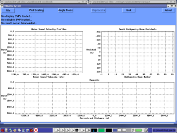
The strategy of mbvelocitytool is to compare an editable SSP with the measured and calculated SSP's we previously collected, and see the effects of our editing in real time on a real data set.

If we first select "File->New editable profile" we'll see a line a line with four (one is hidden somewhat at the top) handles (dots) appear on the "Water Sound Velocity Profile" plot. The handles allow graphical editing of the profile by the "drag and drop" method on the file handles.

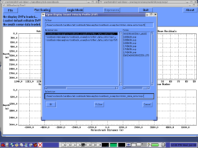
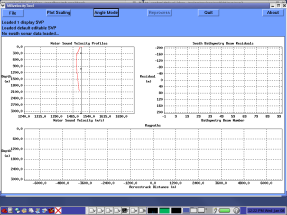
If we select "File->Open editable profile" we'll see a dialog box that will allow us to browse to the location of our sound speed profiles. Find /mbexamples/cookbookexamples/other_data_sets/ssp and load the XBT SSP identifiable by an "sv" suffix. See the figure below:

Figure 4.11. MB-VelocityTool

You'll find the XBT sound speed profile plotted in red on the "Water Sound Velocity Profiles" plot. Why does the data extend down only 2000 meters of water depth? The model of XBT used in this example is good only to that depth, but more importantly, changes in the SSP below the thermocline are entirely due to changes in pressure with depth - so we need not measure much below the thermocline to have a good idea of the shape of the SSP at deeper depths. Here's an illustration:

Figure 4.12. MB-VelocityTool with SSP's Loaded

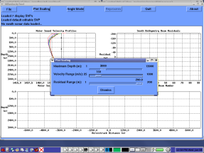
In the same manner as above, load the remaining SSP's generated by mblevitus. They will be added to the plot in various colors to make them easily distinguishable. In an effort to better see the differences between them, we can adjust the scale of the plot by selecting the "Plot Scaling" button. Slide the "Velocity Range" scale to 150. You'll probably be able to see the plot change scale in the background as you let go the mouse. Click "Dismiss" to close the Plot Scaling window.

Figure 4.13. MB-VelocityTool with Plot Scaling Dialog

With out SSP's loaded we can turn to loading our data set. The process is much the same - select "File->Open swath sonar data". Browse to the file, and ensure the correct format is specified in the dialog box before clicking Open. One additional SSP will be calculated for your swath data from the Levitus database automatically. Before we discuss the details of the various plots, let us adjust the plot scaling,"Maximum Depth" to something near 6000 meters. Here is the result:

Figure 4.14. MB-VelocityTool with Sonar Data Loaded

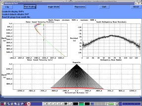
When the loaded sonar data contains raw beam angles and travel times, the path the sonar traveled to the sea floor is calculated and displayed in the "Raypaths" plot. The first good data value in each beam is displayed from the data file (most from the first ping) to allow one to see realtime results of interactive editing. Based on the current SSP a line is fit to the across track profile of each ping and the difference between each bathymetry value and the linear fit is calculated. These are then averaged across the loaded data file and plotted as "residuals" in the upper right hand plot. Bathymetry values that are shallower than the fit are negative while those deeper are positive and the standard deviation of the averages are plotted as error bars.

Next we adjust our editable sound speed profile to approximate the loaded profiles. Place the cursor over one of the handles (dots), click with the left button and drag the profile as is appropriate. Often you will find that the four handles provided are not enough to adequately shape the profile. Additional handles can be added by placing the cursor over the portion of the profile that a handle is desired and clicking the center mouse button. Below the profile has been edited as described.

Figure 4.15. MB-VelocityTool with Edited Profile

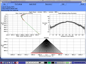
You may have noticed that the ray tracing and residuals plots did not change while we edited our profile. These are updated with a click of the "Reprocess" button. Before we do that however, it will be helpful if we adjust our residual plot scaling. Because our example data set is of good quality, a value of 50 meters is appropriate. Now reprocess the data and note the changes in the Residuals plot.

Here on out, one iteratively adjusts the profile to both flatten the residual plot and minimize the error bars. Meanwhile, the raytracing profile should present a creditable representation of the sea floor.

With the sound speed profile adjusted to your liking, on can save the "editable" sound speed profile by selecting the appropriate choice under the "File" button.

REVISITED WITH A MORE DETAILED DISCUSSION OF THE EDITING PROCESS.

INSERT A DISCUSSION REGARDING SAVING RESIDUALS AND APPLYING THEM TO A DATA SET AND WHEN IT IS APPROPRIATE TO DO SO.