Multibeam sonar systems derive their position information from external navigation systems. These are typically some combination of GPS unit(s) and inertial navigation system(s). Towed sonars and AUV/ROV based systems must use inertial nav systems exclusively (with the exception of an initializing position which is typically correlated to a GPS source). All of these navigation systems are prone to various kinds of error. Multibeam data can only be as good as the reference navigation information the sonar receives.
In an effort to assess the quality of the navigation data, and to minimize its adverse affects on the the sonar data, MB-System™ provides an interactive navigation tool, mbnavedit.
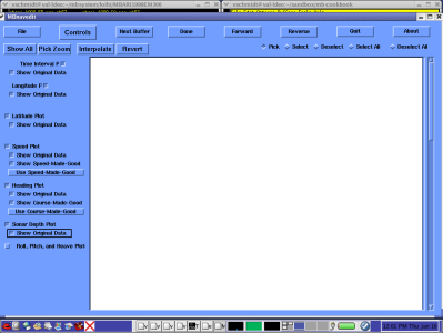
mbnavedit is an interactive tool that loads sonar data files, extracts navigation information, plots that information, and provides a "clickable" tool for editing the data. When swath data navigation has been loaded, mbnavedit displays auto-scaled plots of longitude, latitude, speed, heading, sonar depth time-series and a plot of the difference in time stamps between navigation values. Using these plots, one may clearly identify and correct poor fixes, a loss of heading reference, and even a loss of navigation information altogether.
Note
Navigation of deep-water hull-mounted swath data was poor before GPS and thus required adjustment as well as artifact removal to make overlapping swathes match. Nowadays, the navigation of hull mounted surveys is usually adequate from the start, but navigation of surveys from submerged platforms is almost always initially inadequate.
For surveys from hull mounted sonars, navigation is typically provided by high quality GPS, often augmented by an internal navigation system to provide increased accuracy in heading and smoothing of the fix data.
In contrast, underwater navigation systems generally involve one or a combination of:
Long baseline (LBL): position determined by ranging to an array of transponders.
Ultra-Short-Baseline (USBL): position determined by ranging to a transponder on the ship.
Inertial navigation system (INS): position determined by integrating motion over time using all available data, including acceleration measurements.
There are generally three types of modifications made to the navigation:
Editing: Under most circumstances, the navigation is merely edited. Isolated, obviously wrong values are selected and then replaced by interpolation or by adoption of alternate values (e.g. Course made good for heading or speed made good for speed). Because navigation systems provided to modern hull mounted sonars typically provide very good navigation, a cursory removal of outliers using the direct editing method is usually all that is required.
Modeling: If the position values are totally useless, but good heading and speed values are available, the Dead Reckoning navigation modeling function provided in mbnaveditcan generate a reasonable and self consistent approximation to the navigation. This is sometimes required for deep-towed sonar navigation. If the navigation values are very, very noisy but follow a correct navigation, then the smooth inversion navigation modeling function can generate reasonable navigation that is consistent with the original values. This method is frequently used with USBL-derived ROV navigation.
Adjustment: If the navigation is reasonable, but features don't match where bathymetry and sidescan swathes overlap, then the navigation needs to be adjusted so that these features do match. mbnavadjust is typically used to accomplish this as will be discussed in another section. This step will be required with old, pre-GPS deep water hull mounted data and with modern data from submerged platforms (sometimes even with LBL navigation).
Complicating the sonar-data--navigation-integration problem is that various sonar systems use differing methodologies for storing navigation and time information in their native data files. Some sonar data formats store a navigation record and time stamp with each ping. "Synchronous" data files of this type are the standard for MB-System™ defined formats. Other, sonar data formats, for example those created by Simrad sonars, do not store navigation information with the sonar data files at all. Instead, separate files are recorded for navigation information from up to three sources. Typically recorded at regular intervals, these "asynchronous" data records require interpolation of time and navigation information to the ping times. Still other data formats, such as those produced by Sea Beam 2100 family of sonars produce both synchronous navigation values (associated with each ping), and separate files with asynchronous navigation (at regular intervals).
Caution
Since data file formats such as Format 56 (native Simrad data) have no internal place to put navigation data, converting from other file formats to Format 56 will result in a loss of the navigation data.
To make sense of all of this MB-System™ identifies a "primary" navigation source for each data format type. When synchronous (associated with each ping) navigation data is available it is used. For asynchronous data files, a primary navigation source is chosen and per-ping positions are interpolated from their corresponding time stamps. These distinctions are worth remembering when using mbnavedit. For example, consider the time difference plot which plots differences in successive time stamps for each recorded position. When navigation information is recorded with each ping (synchronously), differences in time intervals correspond to differences in the ping rate. Most sonars automatically adjust the ping rate based on water depth, so one would expect this plot to produce a smooth varied plot (perhaps with jumps where ping rates have been manually manipulated) [Bet you don't have a log of THAT!]. In contrast, when navigation information is recorded separately at regular intervals, one would expect this plot to be, well, regular (constant).
Another distinction worth keeping in mind is the difference between navigation generated from a shipboard sonar and that generated from a transponder or inertial navigation system aboard a towed system, ROV or AUV. In the former, navigation is provided largely by GPS or some other similar navigation source. As such, navigation editing is done to the position data itself, and typically only old sonar data contains navigation so poor that one must smooth through noisy navigation. In contrast, navigation from transponders and inertial systems is generated through integration of acceleration, speed and heading data to generate positional data. In this case, editing is primarily done to the speed and heading data, such that when a dead reckoning algorithm is applied, a more accurate position map is generated.
In addition to the positional Latitude and Longitude information, sonar data formats may (or may not) also store speed and heading. These values are recorded from separate navigation inputs to the sonar system, (in contrast to "speed-made-good" and "heading-made-good" which are calculated from the Latitude and Longitude data). If the speed and heading data are available, mbnavedit plots them, and they may be edited interactively to correct errors. Editing these values and merging them back into the sonar data, however does not change independent position data. It is only when the dead-reckoning algorithm is used to generate position information that the positions recorded for each ping are changed. Editing the "raw" speed and heading data when NOT using the dead reckoning algorithm has no affect on the sonar data grid and is generally a waste of time.
.That said, plotted in blue the heading and speed plots, are speed-made-good and heading-made-good. These curves are generated from successive position information and as such are very sensitive to outliers in the independently generated navigation. They are not directly editable data points, but are very helpful in identifying unruly position data when the dead reckoning algorithm is NOT used.
OK, enough already, let us see some examples.
For illustration purposes, we consider two data files from the Lo'ihi example data set. These files were selected to show navigation typical of both a hull mounted sonar, and a towed sonar. The former is shown to illustrate the application, as there is little editing that is required. The latter is shown to illustrate a particularly difficult navigation problem. First we consider the hull mounted sonar data file.
The mbnavedit process is executed simply by typing the following on the command line:
>mbnavedit
To load a data set, click the "File" button. A dialog box is shown that allows one to browse to find the desired bathymetry or navigation file (as appropriate).
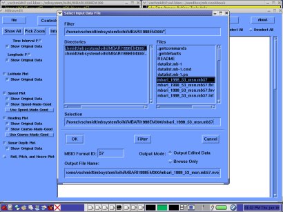
MBIO Format ID is specified in the dialog box at the bottom, as done in mbvelocitytool. Again, this value will be filled in automatically when files are named with the MB-System™ standard *.mb##.
One may also specify, at the bottom right of the dialog box, whether the loaded data will be edited for processing or simply browsed. The former results in creation, on exit, of an edited navigation file as well as a parameter file that will be used by mbprocess to apply the changes. If a parameter file already exists, it will be edited to reference the newly edited navigation file.
The edited navigation file will be created with the base name of the loaded data file plus the ".nve" suffix by default. This naming convention can be changed in the bottom blank where any path and navigation file name may be specified.
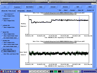
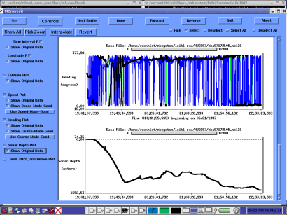
If we select the first EM300 data file of our Lo'ihi data set as is shown selected in the figure above, mbnavedit will load the navigation and produce the plots.
mbnavedit will load all of the navigation information in the file up to a maximum of 25000 records. In the event the file exceeds this number of records, successive chunks of data can be processed by loading successive "buffers" of data without exiting the application and reloading data.
Now lets take a quick look at the plots generated by mbnavedit.
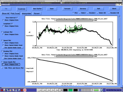
The first are the time interval plot followed by the longitude vs. time plot.
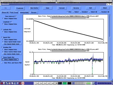
These are followed by the latitude and speed plots:
Scrolling further one finds the heading and sonar depth plots:
As you scan down through the list of plots on the right you'll notice not selected, by default, are plots for pitch, roll and heave. These plots are provided for additional consideration, and can be displayed by clicking on the appropriate button. However unlike the others they are not editable (at the time of this writing). These values are used in the beam forming algorithms of the sonar system and can be helpful in determined causes of irreconcilable errors.
As stated before, editing of navigation data requires different strategies depending on 1) whether the navigation values are from an inertial navigation system (e.g. a towed system, ROV or AUV) or a constant navigation source (e.g. GPS) and 2) whether the sonar stores time information at periodic intervals or with each ping. In the EM300 sonar data file we've chosen to illustrate MBnavedit the primary navigation source is stored synchronously, and since its a hull mounted sonar with a GPS input, we can expect the navigation to be quite good. Just the same, we can use it to illustrate the process.
Let us review the plots shown above and point a few things out.
First consider the time difference or "dT" plot. Remember that time stamps in this data set are integral to the ping data - "synchronous" if you will. Here we see a varying time difference plot that corresponds largely to changes in the ping rate. Spikes in the time interval plot typically reflect abnormal ping cycles rather than a loss of navigation data.
In this particular data file, we have quite a lot of spikes for the first half of the data file, after which the time difference values change in a smooth expected way. There is, in fact, nothing wrong with this navigation data, but these irregular changes in ping rate might be indicative of a different problem that is worth pointing out - an improper configuration of the sonar. Sonars typically require an operator to provide it with a range of depth values (or at least a minimum depth value) in which it should expect to find the bottom. If the sonar had difficulty in reconciling the ping results with this setting (i.e. the actual depth was outside the range) it might attempt to adjust the sonar ping rate frequently, resulting in corresponding fluctuations in this time interval plot. This is likely the cause of the spikes in this plot. A well kept sonar operator's log might provide clues that would alert the sonar data processor for this type of behavior.
As one would expect for a modern, hull-mounted sonar, there is nothing particularly interesting in the Longitude and Latitude plots. They are smooth and continuous. Great! There is nothing to do. Not much of an example. In fact, it is difficult to find hull mounted sonars that require navigation editing. Let us next consider a towed sonar example.
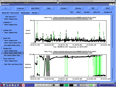
For this illustration we have selected and loaded the first data file from the "HUGO" Loi'hi data set. Let us first review the plots.
First the Time Difference and the Longitude plots:
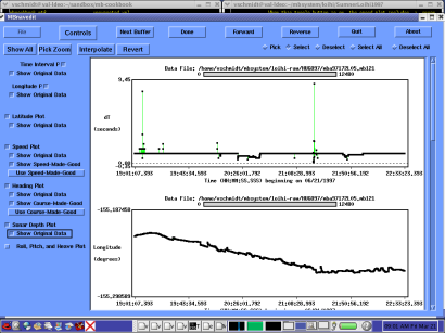
Here we see a nearly constant time difference plot. Navigation is recorded "asynchronously" and ping navigation points are interpolated from the their associated time stamps. A few spikes show blips in the recorded navigation and are inconsequential.
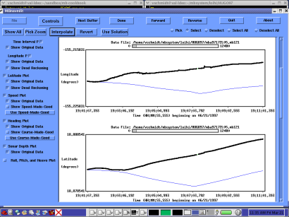
The Longitude plot shows both a "waviness" that we know to be incorrect and more than a few discontinuities. These will have to be addressed in our editing process.
Next the Latitude and Speed plots:
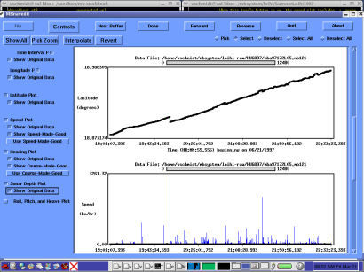
In the Latitude plot, we again see the "waviness" and discontinuities that must be addressed in the editing process. Hints to the errors can be seen in the Speed plot as well. Spikes in the "speed-made-good" plot flag erroneous position data. If we "unselect" the "Show Speed-Made-Good" button we can see that the speed values themselves are quite noisy and are most likely the source of the positional problems.
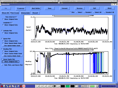
Finally the Heading and Sonar Depth plots:
Here we can see considerable noise in the heading plot. Plus, the blue, heading-made-good plot is a jumbled mess, due to the noise in the position data that we noted earlier. The depth plot is smooth and reasonable and need not be considered at this time.
For a towed sonar of this type, with such poor position data, the general strategy is to edit the speed and heading data, and then recalculate the position data using the Dead Reckoning Algorithm.
First to see the data more clearly, we can remove the speed-made-good and heading-made-good lines from the plot. Simply deselect the "Show Speed-Made-Good" and "Show Heading-Made-Good" toggle boxes on the left.
We can inspect the speed and heading plots more closely using the "Pick Zoom" feature. Clicking the "Pick Zoom" button in the upper left hand corner of the screen changes the cursor to a "+". One may then position the cursor over the plot, aligning it with the left edge of the desired area to zoom and clicking the left mouse button. A red line denotes the edge of the area to zoom. Then one may position the cursor over the right edge of the desired area and click the middle mouse button. A second red lines denotes the right boundary. Positioning the cursor between the two red lines and clicking the right mouse button will zoom the plot to the selected boundaries.

Alternatively, one can manually adjust the horizontal scale. A click of the "Controls" button brings up a drop down menu with "Time Stepping", "Nav Modeling" and "Time Interpolation" options. Selecting "Time Stepping" brings the following dialog:
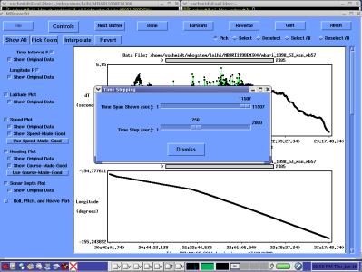
Here the "Time Span Shown" slider allows one to adjust the amount of data that will be plotted in each plot by choosing the time span during which data will be plotted. The default is to plot the entire data set, however for even moderately sized data files this makes editing difficult and one will usually want to adjust this value to a smaller value. Note that this does not translate into the number of data points in any plot, as the ping interval is longer than a second in this data set.
As one "time span" of data is edited one will want to move forward to successive time spans to edit them as well. The shifting of the plots is done by clicking the "Forward" button in the main window, and the "Time Step" slider in this window allows one to specify the amount the plots are shifted with each click. A good rule of thumb is to select a value of about 2/3 of the "Time Span" setting to allow successive shifts in the plot to overlap.
One can now click the "Forward" and "Reverse" buttons in the main window which has the effect of "scrolling" through the plots in time. A white bar with a gray box allows one to see where the current plot is in the larger data set.
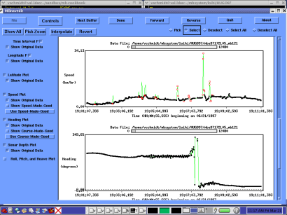
To edit the speed and heading data, we simply select the point or points we wish to edit and click the "Interpolate" button. The original data points are removed and new data points are shown whose values are interpolated from the surrounding remaining data. When "Pick" is selected (at the top right of the mbnavedit window), data points are selected one click and one point at a time. When "Select" is chosen,all the points in the general area of the cursor are chosen and one may "mow" over points by moving the cursor with the left mouse button depressed, selecting everything in the cursor's path. The following illustration shows several points on the speed plot that have been selected and interpolated (on the left) and several more that have been selected, but the Interpolate button has not yet been pressed.
In this way, one continues through the speed and heading plots, removing outliers and smoothing through noisy data. When the process is complete, we then apply the Dead Reckoning Algorithm.
To apply the Dead Reckoning Algorithm, select "Controls" menu, and then "Nav Modeling". At the top of the resulting window, one chooses the kind of Nav Modeling desired, or none at all. If Dead Reckoning was selected, once can select values for Latitude and Longitude drift rates, if known. If Smooth Inversion was selected, one can set weighting factors for speed and acceleration. In this case, we select Dead Reckoning. We will leave the drift rate values blank for this example, HOWEVER, operators of AUV or ROV based sonar systems must maintain a log of local currents such that these corrections can be applied.
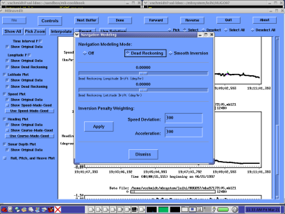
When "Dismiss" is selected to close the window, the "solution" generated by the Dead Reckoning algorithm is plotted in blue on the Latitude and Longitude plots.
Also shown in the mbnavedit is a "Use Solution" button. Clicking this button tells mbnavedit to save the Dead Reckoning solution when exiting such that it may be used as the primary navigation source by mbprocess.