Now that we have done some preliminary work regarding SSP's, physical constants for the sonar system, and navigation corrections, we can begin automated and interactive editing of the bathymetry data itself. Editing of bathymetry in MB-System™ consists simply of "flagging" data points that are erroneous such that they can be ignored. In this way, tools that will later grid the data set, can interpolate from the surrounding data without the interference of poor data points.
It may seem odd that MB-System™ does not allow the user to manually manipulate data points. One cannot look at a piece of sonar data with $mbs; and create one's own sea floor profile through an otherwise noisy data set, as can be done with some sonar data editing systems. Rather, one can only chose existing points to ignore, and allow standard interpolation algorithms to fill in the blanks. The distinction is a subtle, but important difference in philosophy regarding sonar processing on the part of the authors of $mbs;.
Sonar editing, whether automated or manual, creates an ancillary data file, typically with an ".esf" suffix. This binary file contains the list of the data points flagged in the editing process. The depths associated with these data points are given negative values (or zero) during the final processing such that GMT will disregard and interpolate around them.
$mbs; editing processes also check to see if an associated parameter file exits (with the ".par" suffix). If not, one is created. In either case, the parameter file is made to specify the file name of the edits ancillary file, so that it may be applied by mbprocess.
First let us consider automated flagging of Bathymetry.
Lucky for us, many errors in multibeam sonar systems are predictable, such that we can use an automated tool to flag them as incorrect. Toward that end, MB-System™ provides the process mbclean.
mbclean is an extremely useful tool to automate a portion of the bathymetry editing process. Often mbclean can be used in automated scripting to modify sonar data in near real-time such that reasonable quality data can be produced right from the get-go. However, even when processing data from hull mounted, modern sonars, no automated algorithms can approach the discretionary ability of the human eye. Interactive editing with mbedit is recommended to augment the automated editing for publication quality data sets.
mbclean provides seven ways to automatically flag bad beams in the bathymetry data. In the order they are applied, they are:
Flag specified number of outer beams. (-X option)
Flag soundings outside specified acceptable depth range. (-B option)
Flag soundings outside acceptable depth range using fractions of local median depth. (-G option)
Flag soundings outside acceptable depth range using deviation from local median depth. (-A option)
Flag soundings associated with excessive slopes (-C option or default)
Zap "rails". (-Q option)
Flag all soundings in pings with too few good soundings. (-U option)
The first flags a specified number of outer most beams from each side of the sonar. These are commonly poor beams, as SNR is low and sound speed profile errors are magnified.
The second flags sounding outside a specified depth range. This can be helpful when, for example, the sea floor is relatively flat and the range of depths is well known.
Next mbclean optionally flags beams with depths that are outside bounds generated by some specified fraction of the local median depth. This is helpful, when the sea floor is not particularly flat, and depth range is not well known. The local median depth is generated as the median of the current beam and those immediately before and after it.
Then mbclean flags beams that are outside some exact specified range of the local median depth. This option is usually preferable to the previous one when the total depth is quite deep, resulting in larger than desirable bounds using the previous method.
The next method employed by mbclean is flagging based on excessive slopes. This is actually the most common way to identify faulty bathymetry. Four optional methods of flagging beams based on slope are provided. The first flags the beam that is furthest from the local median depth. The second flags both beams associated with the excessive slope. The third method zeroes the beam furthest from the local median depth rather than flagging it. The final method zeroes both beams associated with the excessive slope.
If specified, mbclean will next try to identify groups of along track beams that have abnormally short across track distances and shallow depths. These kinds of errors cause ridges or "rails" along the track of the ship.
Finally, mbclean will toss out entire pings whose quality is so poor that flagging by other methods has resulted in fewer than a specified number of good beams.
We can apply mbclean to a portion of our Loi'hi data set and see how it works. mbedit is such a nice tool for visualizing (and editing as we will see) sonar data, we can use it in this example to see the effects of mbclean. However, the details regarding mbedit are saved for the next section, so for now just bare with me and look at the pictures.
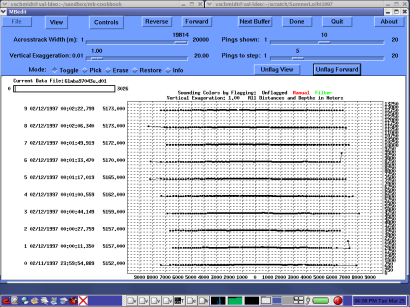
Here is a screen-shot of mbedit with the first data file from the SumnerLoihi data loaded. All flagging of data has been removed the scaling has been adjusted and the data has been scrolled such that erroneous data is easy to make out.
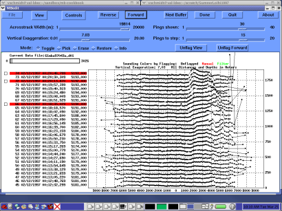
In the screen shot above it is easy to see data that needs editing. In particular, spikes in the outer few beams on either side are apparent. Now lets see if we can clean things up a bit with mbclean.
Normally this would be done in a single step, but for the purposes of illustration we can do them separately to see the results. First let us run mbclean to flag the outer five beams on either side of the swath. This we do with the -X flag.
mbclean -F121 -I 61mba97043u.d01 -X5

Processing 61mba97043u.d01
3026 bathymetry data records processed
14613 outer beams zapped
0 beams zapped for too few good beams in ping
0 beams out of acceptable depth range
0 beams out of acceptable fractional depth range
0 beams exceed acceptable deviation from median depth
0 bad rail beams identified
0 excessive slopes identified
14613 beams flagged
0 beams unflagged
0 beams zeroed

MBclean Processing Totals:
-------------------------
1 total swath data files processed
3026 total bathymetry data records processed
0 total beams flagged in old esf files
0 total beams unflagged in old esf files
0 total beams zeroed in old esf files
14613 total outer beams zapped
0 total beams zapped for too few good beams in ping
0 total beams out of acceptable depth range
0 total beams out of acceptable fractional depth range
0 total beams exceed acceptable deviation from median depth
0 total bad rail beams identified
0 total excessive slopes identified
14613 total beams flagged
0 total beams unflagged
0 total beams zeroed
From the text output, we can see that there were 3026 pings in this data file (each has some 151 beams), and that as a result of mbclean, 14613 beams are now flagged. We can take a look at the file again in mbedit and see what has been flagged.
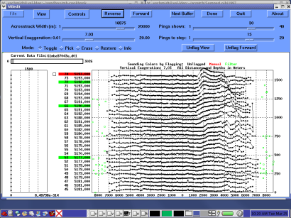
Above we see that the much of the noise in the outer beams has been removed by mbclean.
Perhaps the most common way to use mbclean to automatically flag bathymetry data is to employ the slope checking algorithm. This method is common because sea floor slope is relatively predictable across a wide array of total sea depths. Flagging based on depth limits, set as a fraction or constant portion of the local median depth, often do not produce good results across a large change in the depth of the sea floor, and require flagging in a piece meal way. Slope flagging is specified with the -C flag to mbclean as shown below.
mbclean -F121 -I 61mba97043u.d01 -C1

Processing 61mba97043u.d01
Sorting 14613 old edits...
10000 of 14613 old edits sorted...
3026 bathymetry data records processed
14613 beams flagged in old esf file
0 beams unflagged in old esf file
0 beams zeroed in old esf file
0 outer beams zapped
0 beams zapped for too few good beams in ping
0 beams out of acceptable depth range
0 beams out of acceptable fractional depth range
0 beams exceed acceptable deviation from median depth
0 bad rail beams identified
66280 excessive slopes identified
80893 beams flagged
0 beams unflagged
0 beams zeroed

MBclean Processing Totals:
-------------------------
1 total swath data files processed
3026 total bathymetry data records processed
14613 total beams flagged in old esf files
0 total beams unflagged in old esf files
0 total beams zeroed in old esf files
0 total outer beams zapped
0 total beams zapped for too few good beams in ping
0 total beams out of acceptable depth range
0 total beams out of acceptable fractional depth range
0 total beams exceed acceptable deviation from median depth
0 total bad rail beams identified
66280 total excessive slopes identified
80893 total beams flagged
0 total beams unflagged
0 total beams zeroed
Here we see that mbclean initially processed the flagging we had already applied to the data set. Then the new rules based on a slope of 1 were applied. We can see the results in the following screen shot of mbedit.
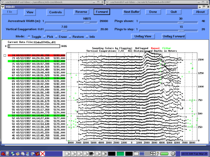
Much is the same as before, but close examination of the small ridge in the upper right hand corner of the data window shows that a few new points have been flagged.
Now there is an error in what we have done in this last step that has been left to illustrate a point. The slope limit of 1 we have chosen in this last step is actually too small (and would be for most data sets). It is not particularly apparent in the screen shot above, however further into the data set, as the Lo'ihi sea mount is approached, the sea floor rises dramatically. The slope limit of 1 flags otherwise reasonable data. Take a look at the screen shot below.
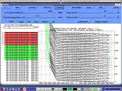
There is a fine line between aggressively flagging of poor data and accidentally throwing out the baby with the bath water. Any setting will suffer from either missing clearly erroneous bathymetry, or flagging data that is actually quite good. It is up to the data processor (YOU!) to assess the data set and choose flagging algorithm parameters wisely. This general method, of trying various slopes or other algorithm parameters with mbclean, and then inspecting the results through the interactive editor, is a good way to quickly get a feel for what parameters might be most appropriate. Experience will bring a better intuition for what works best, and there is comfort in knowing that nothing is permanent. One can always remove the flagging, using mbunclean, and start anew. Again we see that mbclean cannot completely take the place of interactive editing with mbedit.
One of the most useful tools provided by MB-System™ is mbedit. It provides an easy-to-use interface for the interactive editing of sonar data, and several built-in algorithms for the semi-automated editing of data (similar to mbclean). What is more, numerous plots of sonar inputs such as heading, speed, center beam depth, pitch, roll and many others can be viewed right along with the sonar data. The utility of this feature cannot be under stated, as it can be extremely helpful in understanding the causes of poor sonar data and how to fix them.
Cranking up mbedit is quite straight forward:
mbedit
As we've seen in other screen shots, the GUI is much the same as other MB-System™ interactive applications.
Like mbvelocitytool and mbnavedit, the process for loading a data file is much the same. Select the "File" button to generate the "Open Sonar Swath File" dialog box.
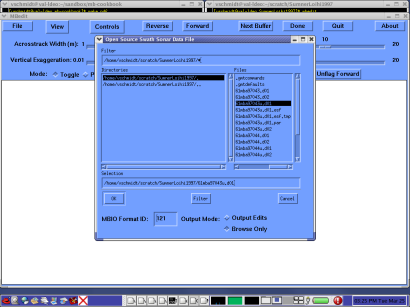
Then simply navigate to the appropriate file to load and select it. Remember to specify the appropriate MB-System™ format ID, and whether you would like to save your editing, or simply browse the data set.
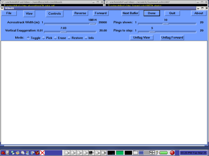
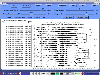
Once loaded the data set will be displayed, one ping at a time, with time stamps to the right as shown below.
Ok, let us look around a bit and make some adjustments to our environment before we get to editing. Plotted on the screen are the first 9 individual pings. In this case, each ping contains 120 beams, and each plot contains 120 corresponding black boxes, plotted on a horizontal scale of athwartships distance and a vertical scale of depth and along track distance. Each box along a ping is connected with thin black lines, as it is difficult to determine their order in noisy data. In this way the plot creates the effect of looking down and forward at the sea floor from the perspective of the sonar.
Across the bottom we see the across-track distance from centerline in meters. Along the left hand side are ping numbers (running from bottom to top), time stamps, and center line depths for each ping. On the right are horizontal distances in meters. At the top left corner of the plot area is a graphical representation of the viewed portion of current data file.
Note that the ping number, timestamp, and depth for the sixth ping in this window are highlighted in red. This indicates that at least one of the beam data points in this ping falls outside the current plot window parameters. We can see this point at the far STBD side of the ping, all the way up in the title of the plot. One may readjust the plot parameters to display all the data, or one may click the small box to the left of the highlighted text to flag the data points falling outside the plot area.
We can adjust the parameters of our plot such that we can more clearly see erroneous data and more efficiently move through the data set. Across the top we have a standard set of buttons which we'll come back to in a moment. Under them are our sliders that allow one to adjust the scaling of the plotted data. "Acrosstrack Width" allows one to adjust he horizontal zoom of the sonar plot, by selecting the maximum distance in the athwartships direction that data will be plotted. Similarly, "Pings Shown" allows one to select the number of pings that are plotted in the window. "Pings to step" simply determines the number of pings that are paged through with each click of the "Forward" or "Reverse" buttons. Finally, "Vertical Exaggeration" amplifies the vertical distances in each ping such that noisy data can be more easily seen.
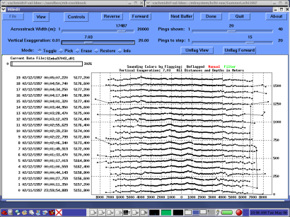
Below I have adjusted the "Pings Shown" slider to 20, the "Pings to Step" slider to 15, and the "Vertical Exaggeration" to 7.
Now let us get on to editing the data.
Much like mbclean, mbedit provides several algorithms to flag erroneous bathymetry data. These can be found by selecting "Controls -> Filters..." at the top of the mbedit window. The "bathymetry filters" window is shown as below.
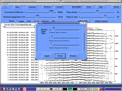
Here we can scroll through several filters that will apply some of the same algorithms provided by mbclean as well as a few new ones. In each sliders are provided that allow one to specify the parameters for the filter.
For example, the "Median Spike Filter" allows one to flag beams whose depths are outside the bounds set as some fraction of the local median depth. (the -G option to mbclean, and the "Flag by Beam Number Filter" allows one to flag a specified number of outer beams (the -X option to mbclean). Appropriate sliders are provided to specify these parameters. "Flag by Distance Filter" allows one to flag data based on their distance from the center beam, and "Flag by Beam Angle" allows one to flag data based on its angle from nadir. The "Wrong Side Filter" numbers each beam from port to starboard and then flags beams whose beam number is higher than the center beam, but sea floor position is to port of it. Beams with the converse scenario are similarly flagged. The slider provided for this filter allows one to specify how many beams surrounding the center beam are ignored by the filter.
To illustrate how it works, I've forward along into the data set so we can see some new data. Here's how it looks:
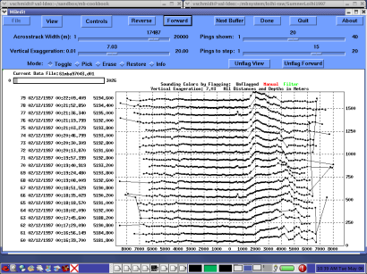
Since the nominal depth is quite deep - 5000m it doesn't make sense to use a fraction of the median depth for our filter criteria. A one percent filter would flag data as high as 50 meters, well within the resolution of most modern hull mounted sonars. So we'll apply the "Flag by Beam Number" instead. For this sonar, the beams are numbered from STBD to PORT, so we slide the sliders appropriately as shown below.
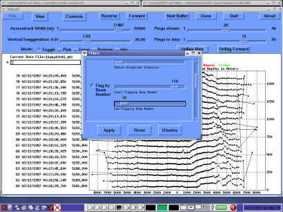
We then click "Apply" and "Dismiss" and the flagged beams are highlighted in green on the display.
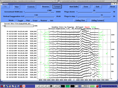
In this case I've flagged 10 beams on either side. This might be too many in this particular case, and will certainly be different from sonar to sonar and environment to environment. Use your best judgment.
One final point to make, the filtering algorithms are applied to data in the current window and to all later data in the file. However they are not applied to data "behind" the current window. If we click "Reverse" we see that the outer 10 beams in the earlier pings have not been flagged by the filter. So if you want to filter the entire file, one must execute the filter with the first pings showing.
There are several modes that we can place the cursor in for "point and click" editing. These are specified using the toggle buttons next to "Mode" in the mbedit window. The first is "Toggle" mode. In this mode the cursor can be placed over any data point and a click will flag the point. A second click will "unflag" the point. This mode is great for precise editing of individual beams. Similarly, "Pick" will also flag an individual beam, however, a second click will not "unflag" the beam. This allows greater control of beam flagging without accidentally undoing your work. "Erase" mode allows one to drag the cursor over data points to flag them, rather than clicking each time. While not as exacting as the earlier modes, "Erase" mode can be much less tedious. "Restore" is similar to "Erase" in that flagged beams can be "unflagged" by dragging the cursor across them. And finally, "Info" is not an editing mode at all, but displays loads of information about each selected ping.
To demonstrate, I've scrolled backwards in the data set to an "unfiltered" portion. The unedited data is shown below.
Now using the Toggle Mode, I can select several beams that need editing. In comparing the previous figure and the following one you will find that the lines connecting across track beams interpolate around flagged data points. You'll also see the flagged data points in read, indicating that they have been manually flagged.

In this way, one can page through each data file, inspecting the sonar data and throwing out data that appears unreasonable.
When exiting the mbedit, an ancillary ".esf" file is created that contains the edited data points. To ensure that this new ".esf" file is used in the final processing step, the ancillary processing parameter file is automatically edited to reference it. If the ".par" file does not yet exist from other preprocessing steps, it is created.
With the automatic and interactive editing of the bathymetry complete, one can turn to preparations for processing of the sidescan data.