Simulation of production and elastic properties of reservoirs to validate time-lapse seismics.
Simulation of production and elastic properties of reservoirs to validate time-lapse seismics.
Any reference should be made as "Guerin, Gilles 2000. Acoustic and Thermal Characterization of Oil Migration, Gas Hydrates Formation and Silica Diagenesis, PhD. Thesis, Columbia University"
Time-lapse, or 4-D, seismic monitoring is an integrated reservoir exploitation technique based on the analysis of successive 3-D seismic surveys. Differences over time in seismic attributes are due to changes in pore fluids and pore pressure during the drainage of a reservoir under production. The detection of areas with significant changes or with unaltered hydrocarbon-indicative attributes can help determine drilling targets where hydrocarbons remain after several years of production.
Making sure that seismic differences are related to fluid flows is critical for a complete time-lapse seismic study. Differences in data acquisition, survey orientation, processing and quality of datasets can introduce significant noise in the 4-D analysis. This can be especially true when legacy datasets are used, which were not acquired specifically for 4D interpretation. Also, to quantify the amount of hydrocarbons responsible for the seismic differences, it is necessary to have a complete petrophysical model of the reservoir to establish a direct relationship between seismic attributes and pore fluids. Such a model can be built by stochastic simulations of the lithology and porosity, which are dependant on the availability and spatial distribution of the well data that are used as reference. Both, the 4D seismic analysis and the petrophysical characterization, require an independent validation or calibration.
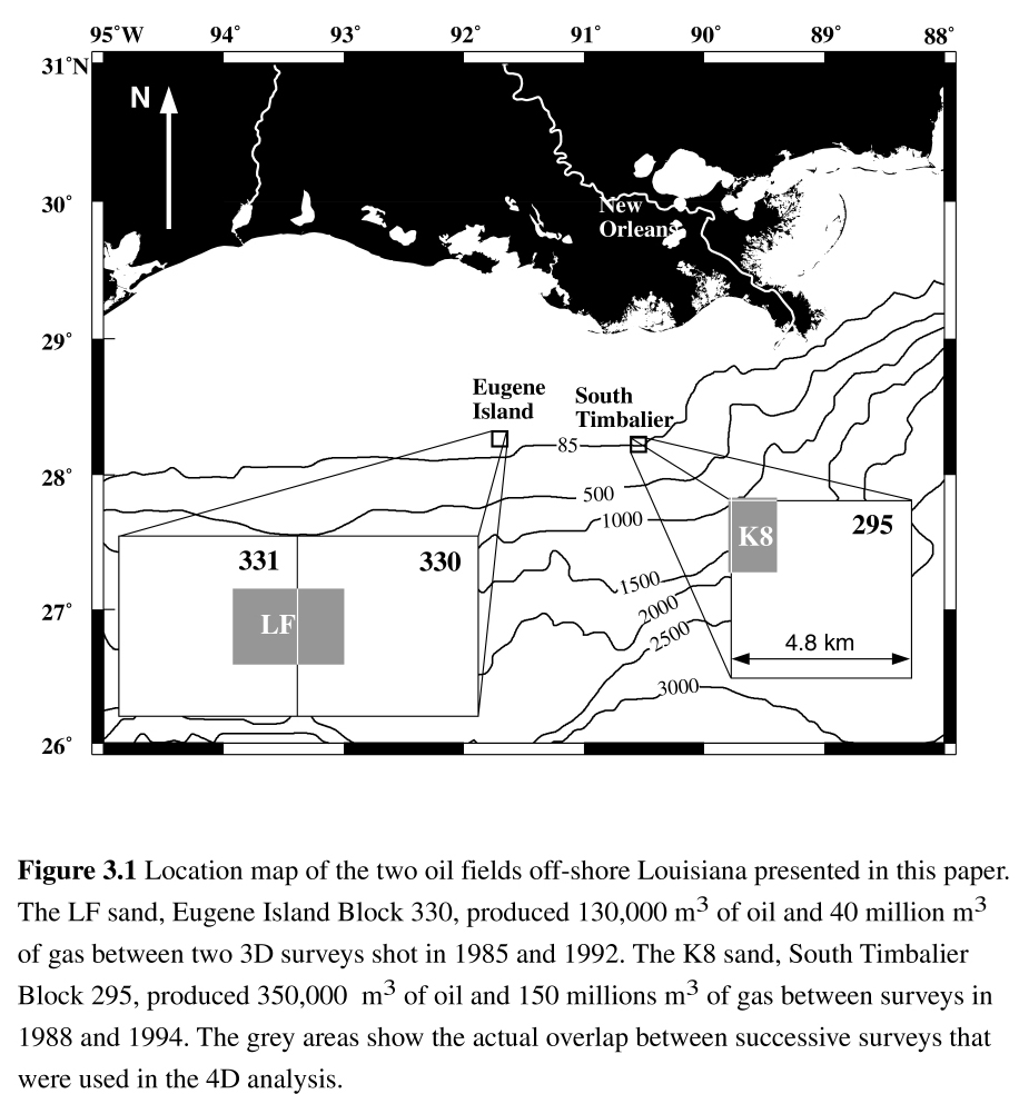
In this paper, we describe how reservoir simulation can be used to generate independent impedance maps to validate or constrain time-lapse interpretation of legacy data sets. A complete 4D analysis is an iterative loop where the original interpretation can be refined along the way. First, we summarize the steps preceding the reservoir simulation, including the 3D seismic processing and inversion, and the preliminary time-lapse interpretation. We then describe the elastic models, the properties of reservoir fluids and the reservoir characterization that are used to link the impedance volumes to fluid and lithology distribution in the reservoir. A comparison with impedance maps derived by these equations from simple vertical fluid substitution shows how the observed 4D differences indicate complex migrations that require a realistic reservoir simulation. After description of the reservoir simulator, the results of the simulation are finally used to generate impedance maps that can be compared with seismic inversions. To illustrate the different steps of the entire procedure we use the case study of the K8 reservoir, South Timbalier 295, because of its relative simplicity. In the last section, we present a complete 4D analysis of the Eugene Island 330 field whose complex history is representative of enduring Gulf Coast reservoirs (Figure 3.1)
|
|
 |
The first steps of the 4D "loop" are described in great details by He [1996] and are only summarized here to define the starting point of the reservoir simulation and lithological model used in the simulation.
3.2.1 Registration and normalization of seismic datasets
Until recently, no seismic survey was shot with the specific purpose of time-lapse analysis. Successive data sets over one location were usually collected with different spacing and orientation. In order to differentiate the seismic attributes (amplitude or impedance) between two surveys, it is first necessary to re-locate them on the same grid. This re-location process uses a 3-D interpolation algorithm, that interpolates between the two grids in travel-time, slice by slice. In addition, in order to be able to compare the results of the inversion of two datasets, we perform a normalization of the amplitudes of the surveys, globally with respect to each other first, and by rescaling them both to a proper amplitude by using synthetic seismograms generated from velocity and density logs acquired in the same area [He, 1996]
3.2.2 Non linear inversion of successive 3D datasets
Standard 3D seismic interpretation uses generally seismic amplitudes to identify reservoirs. Time-lapse analysis performed on seismic amplitudes has also been shown to allow the identification of migration pathways [He, 1996]. However, amplitudes are only proportional to seismic reflectivity, which depends on the relative variability in the elastic properties of the formation, not on the value of these properties. The comparison of 3D amplitude volumes requires wavefield envelope comparison techniques to identify the high-gradient envelop surrounding High Amplitude Regions [He, 1996, Anderson et al., 1994] that have to be identified for time-lapse interpretation.
In contrast, seismic impedance (Z) is directly related to the elastic properties of the sediments :
Z = rVp (1)
where r is the bulk density and Vp the sonic compressional velocity. r is the volumetric average of the density of the different phases (fluids and solids) and Vp can be explicitly expressed as a function of their density and compressibility (see later sections). Also, unlike amplitudes, a simple algebraic subtraction between the impedance volumes at two dates can be directly converted into fluid or pressure changes. A 4-D analysis based on impedance volumes allows a direct qualitative interpretation of seismic changes in terms of fluid substitution or migrations [He, 1996].
He [1996] uses a constrained non-lineal inversion technique to estimate the acoustic impedance volumes from each 3D survey. After the seismic datasets have been horizontally stacked, migrated and re-located, each seismic trace is considered as a one-dimentionnal zero-offest trace. The one-dimensionnal non-linear inversion uses a forward convolution model to compute seismic traces from impedance functions. The implementation of the inversion is based on a modified Levenberg-Marquardt minimization algorithm [More, 1977]. The procedure his made fast and robust by using log-derived impedance trends as a priori impedance functions, and by using covariance functions to constrain the objective functions that are minimized during the inversion [He, 1996].
3.2.3 Preliminary 4D interpretation of the K8 sand
To illustrate the methodology, we present the results of the successive steps of the 4D analysis of the K8 reservoir in the South Timbalier 295 field, offshore Louisiana (See figure 3.1 for location). It is the uppermost of the three most productive reservoirs in the ST295 field and produced about 350,000 m3 of oil and 150 millions m3 of gas between two 3D surveys shot in 1988 and 1994.
| Figure 3.2 |
 |
The K8 sand (Figure 3.2) is a
combination of channelled mid-fan sheet sands lapping on a paleo-high in
the east and gently dipping to the South West [Hoover, 1997]. It
represents a particularly suitable case study in 4D analysis for several
reasons: (1) the first 3D seismic survey was shot before production started,
providing a reference seismic volume where fluids in place are in hydrostatic
equilibrium. (2) The second survey was shot after 5 years of intense production,
which should generate profound changes in pore fluid distribution and pressure
over the reservoir. (3) Only two wells have been producing between the
two seismic surveys (Figure 3.3), which should allow for a relatively simple
migration pattern identification in the 4D seismic.
| Figure 3.3 | 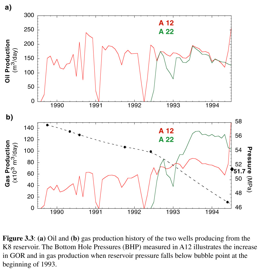 |
Figures 3.4a and 3.4b show the
results of the inversion of the two surveys shot in 1988 and 1994 over
K8. The various layers displayed, numbered from top to bottom, follow the
structure of the reservoir shown in Figure 3.2b. Each layer has 101´
101 data points, distant by 12.5 m and 20 m in the EW direction and NW
direction, respectively, which corresponds to the resolution of the seismic
grid after re-location of the two surveys. The difference between the two
inversions (Figure 3.4c) shows a global decrease in impedance (red) in
most of the shallower layers and updip (NE) from the two producing wells
in the deeper layers. Impedance has mostly increased (blue) in the deeper
layer of the reservoir between the two surveys. Because the reservoir was
originally filled with oil, and the replacement of oil by gas or water
respectively decreases or increases the density and the sonic velocity
of the formation, Eq. (1) allows a preliminary qualitative interpretation:
oil might have been replaced mostly by gas in the shallower layers of the
reservoir and by water in the deeper layers. The substitution of oil by
gas exsolution updip is controlled by the pressure decrease induced by
the producing wells (see pressure drop in Figure 3.3b), while the
replacement of oil by water in the deeper layers is assisted by the presence
of an aquifer supporting the reservoir [Tucker, 1997, Mason,
1992].
| Figure 3.4 | 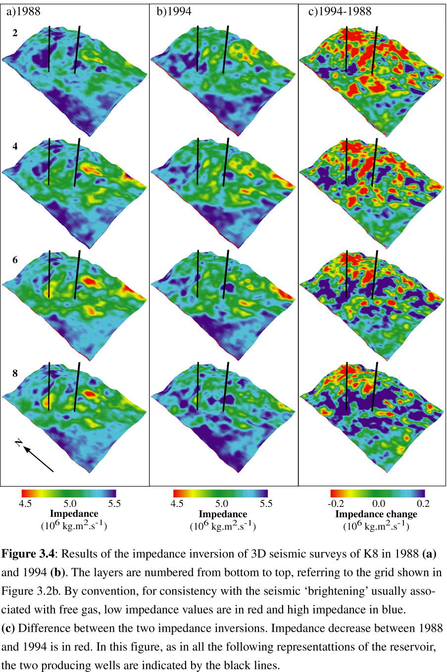 |
Independently of the nature of the pore fluid, the bulk of the impedance of such medium porosity sediments (40% maximum) is controlled by the porosity and lithology distributions. To relate quantitatively the observed changes in impedance with the nature and the volume of the pore fluids, it is necessary to have a complete representation of the sediment matrix, and to define the relationships between the different component of the system and its elastic properties.
3.3 Elastic properties of reservoir sediments
Explicit relationships relating pressure, pore fluid, porosity, matrix materials and the elastic properties of marine sediments have been the topic of many studies, some theoretical [Gassmann, 1951, Biot, 1956, or Kuster and Toksöz, 1974], some empirical [Han et al., 1986, Ramamoorthy et al., 1995, Tosaya and Nur, 1982]. They are all limited in application by the infinite number of parameters affecting the elastic properties of sediments and no approach can offer a comprehensive formulation. We reviewed some commonly accepted models and relationships that could be used to link the changes observed in our impedance maps with fluid substitutions in the reservoirs. Most of them define relationships for the elastic moduli of the formation instead of the impedance. The bulk modulus (K) is the inverse of compressibility and the shear modulus (G) is a measure of the shear strength. Compressional and shear (Vs) sonic velocity can be expressed as functions of these moduli and of the density of the sediments:
![]() (2a) and
(2a) and ![]() (2b)
(2b)
and the impedance can be re-written
![]() (3)
(3)
3.3.1.1 Theoretical formulations
Gassmann [1951] and Biot [1956] expressed the bulk modulus of fluid-saturated sediments as a function of the bulk moduli of the dry frame (Kf), of the pore fluid (Kfl) and of the grains (Kg)
![]() with
with ![]() .
(4)
.
(4)
This formulation requires the knowledge of the dry bulk modulus, for which Hamilton [1971, 1982] established empirical relationships as a function of porosity for several types of lithology. Using his results for clay, silts and fine sands, we define a single formula for clastic sediments:
log (Kf) = log(Kg) - 4.25F or log(Kf/Kg) = - 4.25F. (5)
The grain modulus of a shale/sand mixture can be calculated by a Voigt-Reuss-Hill average of the grain moduli of sand (Ks) and clay (Kc) [Hamilton, 1971]:
![]() (6)
(6)
where g is the shaliness or volumetric shale fraction. We refer to it as the Gassmann/Hamilton model [Guerin and Goldberg, 1996, Chapter 2]. Values of the grain moduli are given in Table 1.
Kuster and Toksöz [1974] used the theory of sonic waves scattering and propagation to calculate the effective elastic moduli of a two phase medium made of spherical inclusions in a uniform matrix:
and ![]() (8)
(8)
Unlike the Gassmann/Hamilton model, Eqs. (7) and (8) do not require an empirical expression of the dry modulus, and for this reason could seem of a more practical use. This model (KT) also offers a relationship for the shear modulus, which is required to calculate Vp and the impedance but is not provided by Gassmann/Hamilton. However, it depends on strong assumptions on the shape and arrangement of the grain that can be of limited relevance to describe the grains configuration of the rapidly buried Gulf Coast sediments.
3.3.1.2 Experimental relationships
Underlining the practical limits of these theoretical relationships, particularly regarding the specific influence of clays on sonic wave velocities, Han et al. [1986] used shaly sandstone core samples presenting a wide range of porosity and shaliness to define in laboratory the following linear relationships between ultrasonic velocities, porosity and clay content:
Ramamoorthy et al. [1995] note that (9) and (10) and other similar empirical linear relationships fail to describe properly the elastic properties of shaly sediments in some standard lithological conditions. They propose to consider independently the effects of porosity and clay. Using in situ data from shear sonic and geochemical logs they give the following relationship for the shear modulus of shaly sediments:
with Ggrain = (0.039log10(g) + 0.072)-1 (12)
Knowing the limits of any of the above relationships we have to determine which one could be used the most reliably and the most readily for the qualitative interpretation of the time-lapse impedances maps in an integrated 4D analysis. In addition to the properties of the matrix, this requires to formulate also the elastic properties of the pore fluid, which are the primary parameters responsible for changes in impedance during production.
3.3.2.1 Properties of fluid mixtures
The elastic properties of the pore fluid are in fact the properties of a fluid mixture, which is a function of the properties of the various fluid phases. The three primary types of pore fluid in a reservoir are hydrocarbon gas (gas) hydrocarbon liquid (oil), and brine. The density and the compressibility of the mixture are the weighted averages of the three phases:
Soil + Sgas + Sbrine
= 1
(13)
rfluid =
Soilroil
+ Sgasrgas
+ Sbrinerbrine
(14)
![]() (15)
(15)
3.3.2.2 Elastic properties of reservoir fluids
Batzle and Wang [1992] give a detailed description of the properties of reservoir pore fluids and we only summarize the parameters and principal relationships that can be used in time-lapse analysis. Physical properties of reservoir fluids are dependant on composition, pressure and temperature. Unless thermal recovery techniques are used, the variations of temperature in a reservoir are negligible during its production history, and pressure and composition are the dominant parameters affecting the changes observed between two surveys.
Brine: Brine physical properties are extremely dependant on its salinity (S). In the Gulf of Mexico, the presence of the buried Jurassic salt generates a significant increase of salinity with depth. In most reservoirs, brine samples are collected and their salinity measured, but Batzle and Wang [1992] offer a relationship to estimate salinity as a function of depth that can be used for gulf coast sediments. They also provide relationships for the velocity and density of brine as a function of salinity, pressure and temperature (See Appendix). Brine density and velocity increase with pressure in standard hydrocarbon reservoir conditions.
Gas: The gaseous phase present in the pore space of a reservoir is a mixture of the lightest hydrocarbon fractions. Its composition can vary during production when reservoir pressure decreases and the lightest oil components come out of solution. The properties of the gas mixture can be characterized by the gas specific gravity (G) measured at standard temperature and pressure conditions (15.6° C and 1 atm). If a complete PVT (Pressure-Volume-Temperature) analysis of the physical properties of gas samples is not systematically performed, the measure of its gravity is most often available and allows a good estimation of its properties as function of pressure and temperature [Batzle and Wang, 1992]. The formulas in the Appendix show that the density and the bulk modulus of gas mixtures increase significantly with pressure.
Oil: The elastic properties of the `Oil' phase, or liquid hydrocarbon, are the most complex of the reservoir fluids, but can also be calculated from a few experimental parameters [Batzle and Wang, 1992]. In addition to the crude oil produced at the surface, the oil phase in a reservoir can include dissolved light hydrocarbons that are gaseous at lower pressure. One of the key parameters controlling the properties of oil is the bubble point pressure, which is the maximum pressure where free gas can be present. As long as reservoir pressure is above bubble point, oil is under-saturated with regard to gas, its composition remains fixed and the density and bulk modulus both increase with increasing pressure. If reservoir pressure falls below bubble point during production, the lightest dissolved gas start coming out of solution. As pressure decreases and more light component leave the liquid phase, only the heaviest hydrocarbon remain in this phase, and the density and bulk modulus of the oil phase increase with decreasing pressure [Batzle and Wang, 1992, England et al., 1987].
The value of the bubble point and the relationships between pressure and elastic properties should be determined from PVT analysis of actual oil samples. If such analysis is not performed, the values of oil and gas density at surface conditions can be used to determine these relationships and the bubble point pressure [Batzle and Wang, 1992, Beggs, 1992 , see equations in Appendix].
One of the standard indicators of fluid properties is the produced Gas-Oil ratio (GOR), which is the ratio of the volumes of gas and oil produced at the surface. The GOR remains constant as long as the reservoir pressure is above bubble point, but increases as soon as pressure falls below this value and free gas saturation exceeds a critical value, at which point it becomes mobile and gets preferably produced [Batzle and Wang, 1992, Steffensen, 1992]. This is shown clearly in K8 (Figure 3.3b) by the rapid increase in gas production in well A22 at the beginning of 1993 when reservoir pressure fell below the bubble point at 51.7 MPa. The evolution of the GOR is one of the key control parameters in monitoring production simulation.
3.3.2.3 Original fluids in place
The last aspect of fluid properties affecting the impedance volume is the distribution of the different phases within the reservoir. While one of the goals of the reservoir simulation is to determine the evolution of these distributions during production, the original fluids in place before production can be totally determined from the fluid PVT properties if we assume the reservoir in hydrostatic equilibrium. The density-pressure relationships provide the pressure gradient within each phase and the entire pressure and fluid distributions can be integrated from the knowledge of the depth of the oil-water contact (OWC) and of one pressure value at one depth within the oil or gas zone. Additional parameters necessary for the most accurate distribution include capillary pressures between each phase and the connate water fraction, or irreducible water saturation, which depends on matrix properties and is measured on reservoir samples.
In the case of
K8, the original oil-water contact in 1988 was detected at 3350 mbsf, downdip
from the study area. The Bottom Hole Pressure (BHP) measured in A-12 at
the beginning of production was 57.7 MPa. These two data points and the
oil gravity (define the pressure distribution at equilibrium shown in Figure
3.5.
| Figure 3.5 | 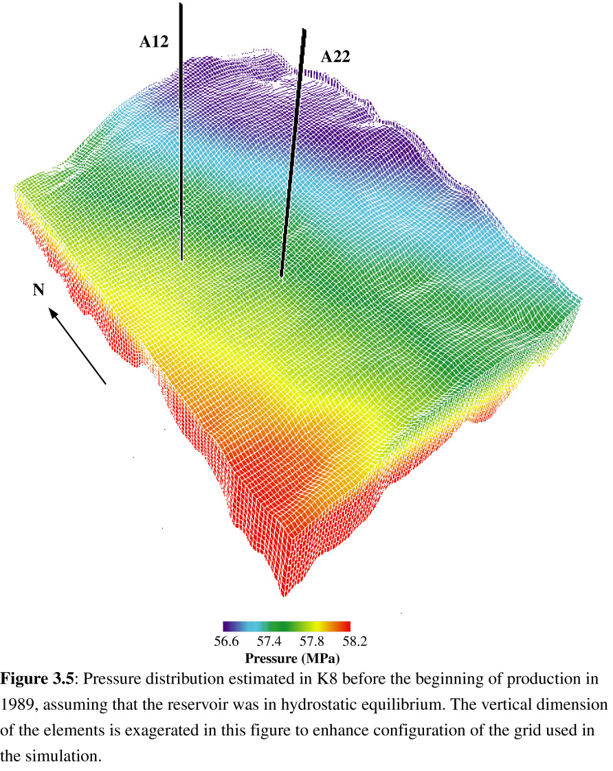 |
Because the lowest pressure was higher than the bubble point (51.7 MPa ) no gas was present. Because the OWC was deeper than the lowest point in the study area, water saturation was uniformly equal to the connate water fraction [30%, Hoover, 1997] and oil occupied the rest of the pore space (70%).
3.3.3 Stochastic reservoir characterization
The missing link between impedance volumes, fluids properties, saturations and pressure distribution using equations (1)-(15) resides in the characterization of the reservoir porosity and lithology distribution. We use geostatistical simulations for this characterization, assuming that within an individual reservoir petrophysical and acoustic properties are closely related and can be associated with calibrated cross-correlation functions [He, 1996]. Using well logs as "Hard" accurate data and impedance volumes as "Soft" data, this method combines the high vertical resolution and accuracy of logs with the wide aerial coverage of 3D seismics. He [1996] provides a complete description of the Markov-Bayse conditional soft indicator technique used .
The lithology is expressed in terms of shaliness. The hard data are shale fraction values calculated from Gamma Ray (GR) and Spontaneous Potential (SP) logs in wells distributed across the reservoir. The soft "inaccurate" data, which have to be of the same type, are approximate shaliness values (gs) calculated from the impedance volume by a simple weighted average:
| Figure 3.6 | 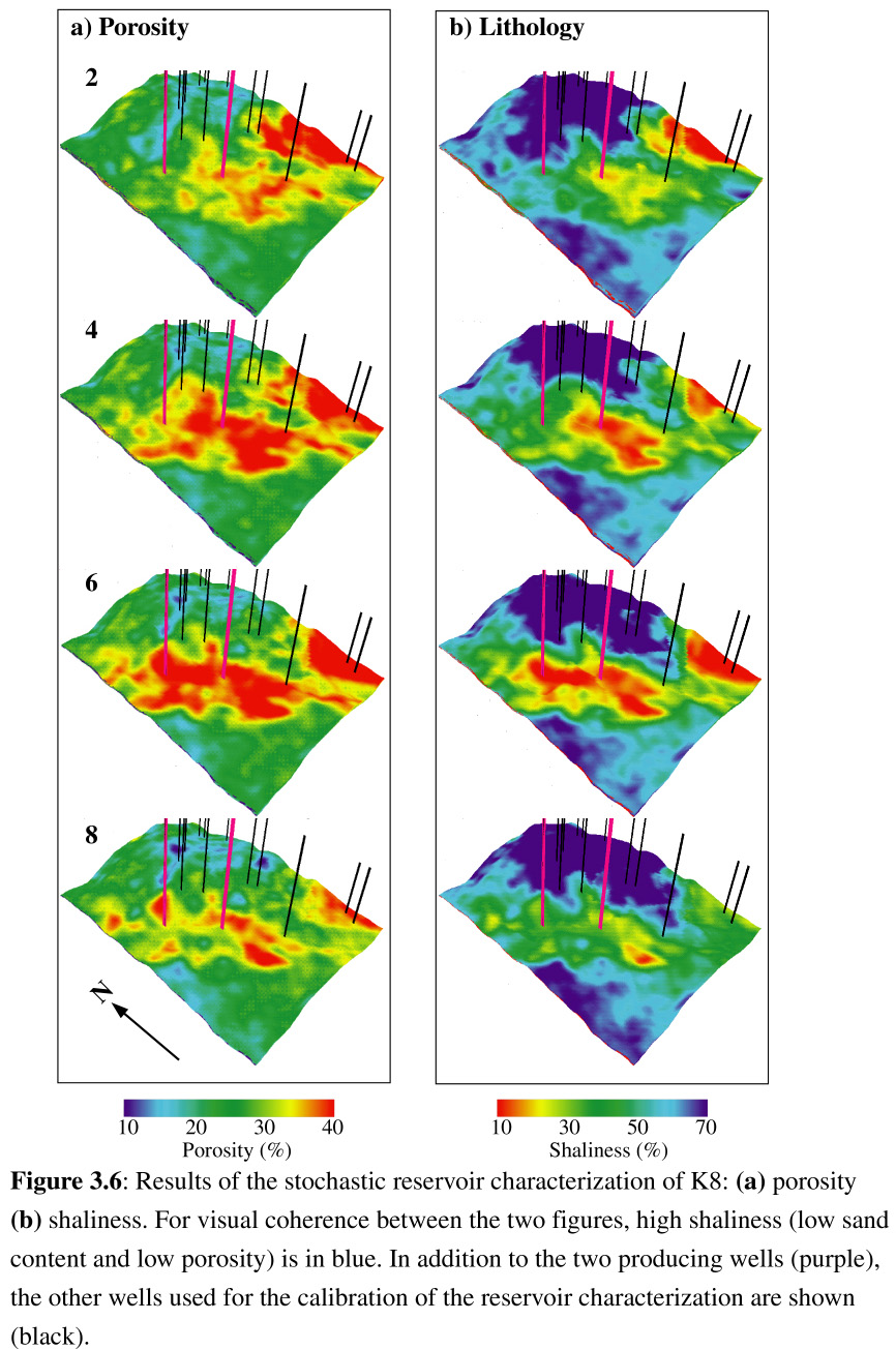 |
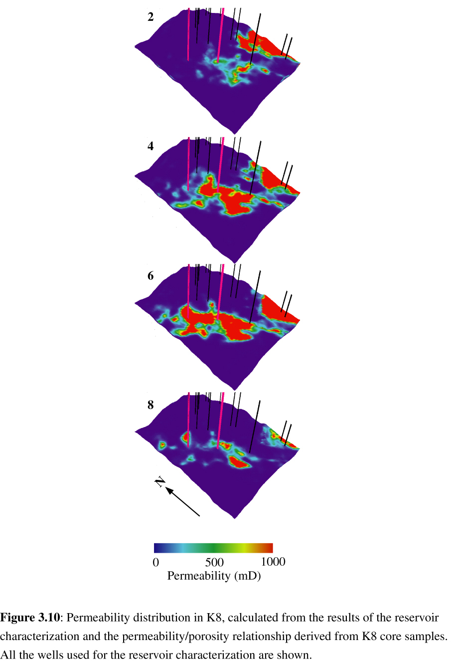
Sixteen wells provided the hard data used to constrain the reservoir characterization of K8 (figure 3.6). Both porosity and shale distributions show a high level of heterogeneity, illustrating the channelled deposition of the reservoir. The bulk of the porosity is located immediately downdip from the two producing wells and in the South East corner of the study area.
3.3.4 From saturation to impedance
The reservoir
characterization allows to use any of the petrophysical models (Eqs 4-10)
to calculate the impedance volumes when pressure and fluid distributions
are known. Having previously established the fluid and pressure distribution
before production in K8, we can compare the estimations of the different
models with the 1988 impedance inversion to determine which formulation
offers a better representation of the observed reservoir properties. Since
the Gassmann/Hamilton model (Eqs 4-6) does not provide a value for the
shear modulus, we combined this bulk modulus estimate with the shear velocity
or moduli expressions of Han et al. [1986](Eq. 10), Kuster and Toksöz
[1974] (Eq. 8), and Ramamoorthy et al. [1995] (Eq. 11) to estimate
three different impedances values. We refer to these values as the Gassmann+Han,
Gassmann+KT and Gassmann+Ramamoorthy impedances, respectively. Two additional
impedance volumes were calculated with the complete KT model (Eqs. 7-8)
and with the expression of Vp and Vs given by Han
et al., [1986] (Eqs 9-10). We refer to these values as the KT and Han impedances,
respectively. All the parameters used for grain and fluid properties are
given in Tables 1 and 2.
| Figure 3.7 | 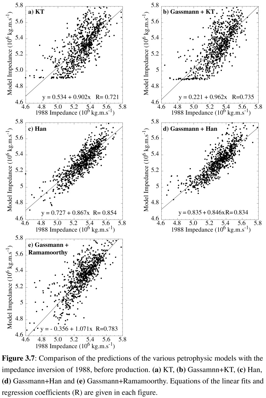 |
In Figure 3.7, the crossplots of the different models with the 1988 impedance allow to compare their respective validity. In all these figure, a perfect formulation should result in an identical linear fit with the inverted values. The KT and Gassman+KT impedances (Figs 3.7a and 3.7b) display the highest level of scattering and consequently the poorest agreement with the inversion results. The Han and Gassmann+Han impedances present the best agreement with the inversion, with regression coefficients higher than 0.80. This comparison seems to indicate the better readiness of these two formulations to represent the acoustic properties of the reservoir in hydrostatic equilibrium. The impedance distribution calculated with Gassmann+Han is shown in Figure 3.8a and compares very well with the 1988 inversion (Fig 3.4a). It will be necessary, however, to make a similar comparison after simulation to evaluate how fluid substitution affects the comparison between the calculated and the inverted impedance.
3.3.5 Comparison with vertical sweep
This preliminary
validation of the elastic formulations can be used to illustrate the need
for an accurate understanding of the reservoir dynamics that time-lapse
seismic can provide. A traditional view of the fluid movements within a
producing reservoir is of a uniform buoyancy-driven movement of the different
phases, the contact surfaces between adjacent phases remaining horizontal.
In the case of K8, where the driving mechanisms are gas ex-solution and
a weak aquifer support [Mason, 1992], this would mean that the gas/oil
contact (GOC) migrates uniformly downdip, as the gas cap expands and more
gas come out of solution, while the WOC progresses upwards. Because the
BHPs measured in the two wells after 1992 were below the bubble point,
this indicates that the GOC has migrated down to at least these depths
(3250 mbsf). Assuming that the GOC and WOC have been simply sweeping uniformly
along dip, and that the reservoir is still globally in hydrostatic equilibrium
at any time, we have calculated as previously the pressure and fluid distribution
that would exist in 1994 if an horizontal gas cap had formed down to 3280
mbsf and the WOC had moved up to 3320 mbsf. The impedances calculated from
these values using the Gassmann+Han formulation are shown in Figure 3.8b.
| Figure 3.8 | 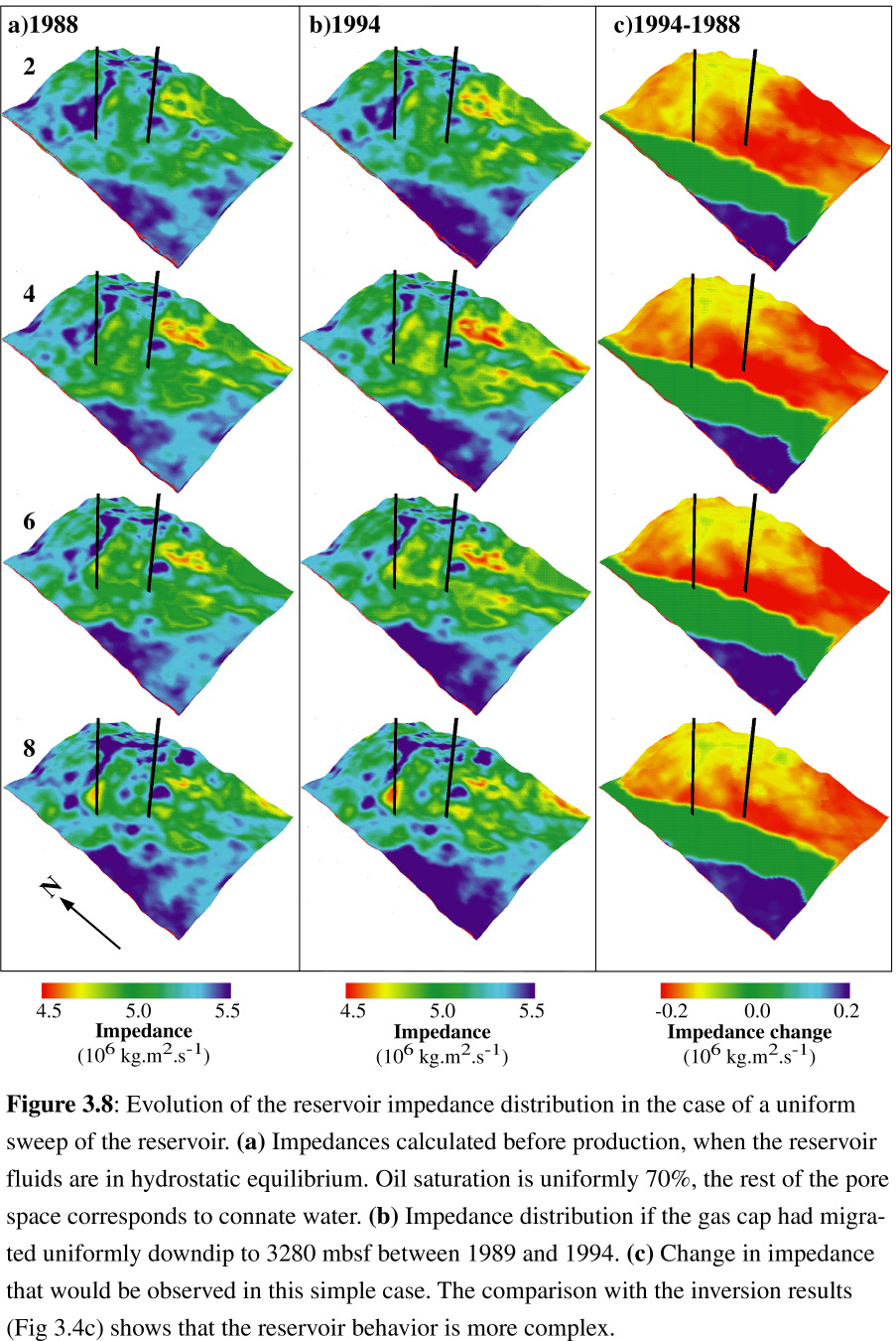 |
Comparison with Figure 3.4b shows that the impedances calculated present strong similarities with the 1994 inversion results. The impedance changes over time (Figures 3.4c and 3.8c) also display some global similarities: decrease in impedance updip from the wells, and increase downdip. However, the pattern and the absolute values of the observed impedance changes are much more heterogeneous in Fig 3.4c than in this simple `gravitational sweep'. The bright areas in the observed impedance changes correspond to isolated impedance decreases, that could indicate areas with low connectivity where hydrocarbon, mostly gas, would remain trapped as the reservoir pressure decreases. The comparison of Figs 3.4c and 3.8c shows that after a few years of intense production, the representation of a GOC as a continuous horizontal surface is merely irrelevant. The fact that the impedances calculated after the reservoir sweep (Fig 3.8b) compare reasonably well with the inversion results in 1994, despite the major differences in the changes over time (Fig 3.4c vs. Fig 3.8c), shows how crucial it is for each inversion to be the most accurate, as differentiating between the inversions of successive surveys is much more sensitive to errors than either inversion.
The entrapment of hydrocarbons is mostly the result of the heterogeneity in the reservoir and in the permeability distribution. Assuming that our inversion results are correct, the heterogeneity observed in the impedance difference over time suggests a migration process more complex than the simple gravitationnal sweep. Numerical simulation of the migration of the different phases can be used to identify the actual behavior of the reservoir under production.
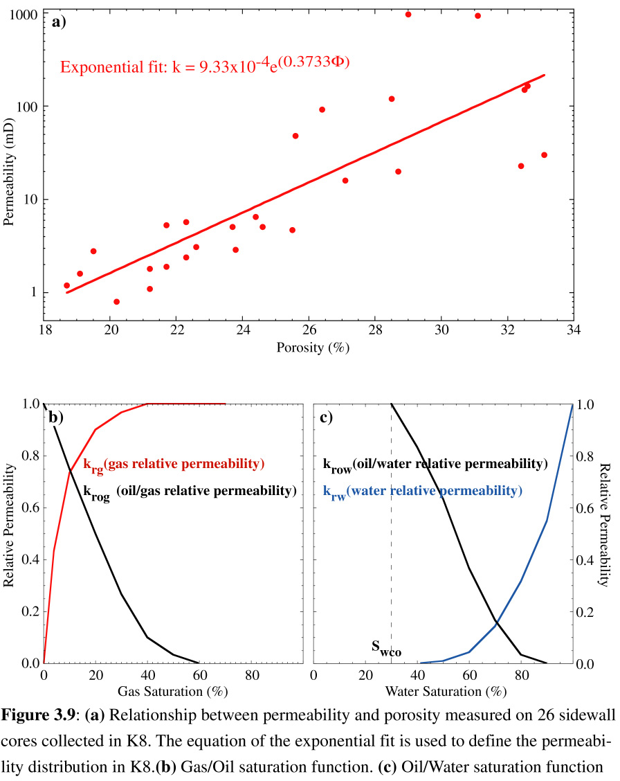
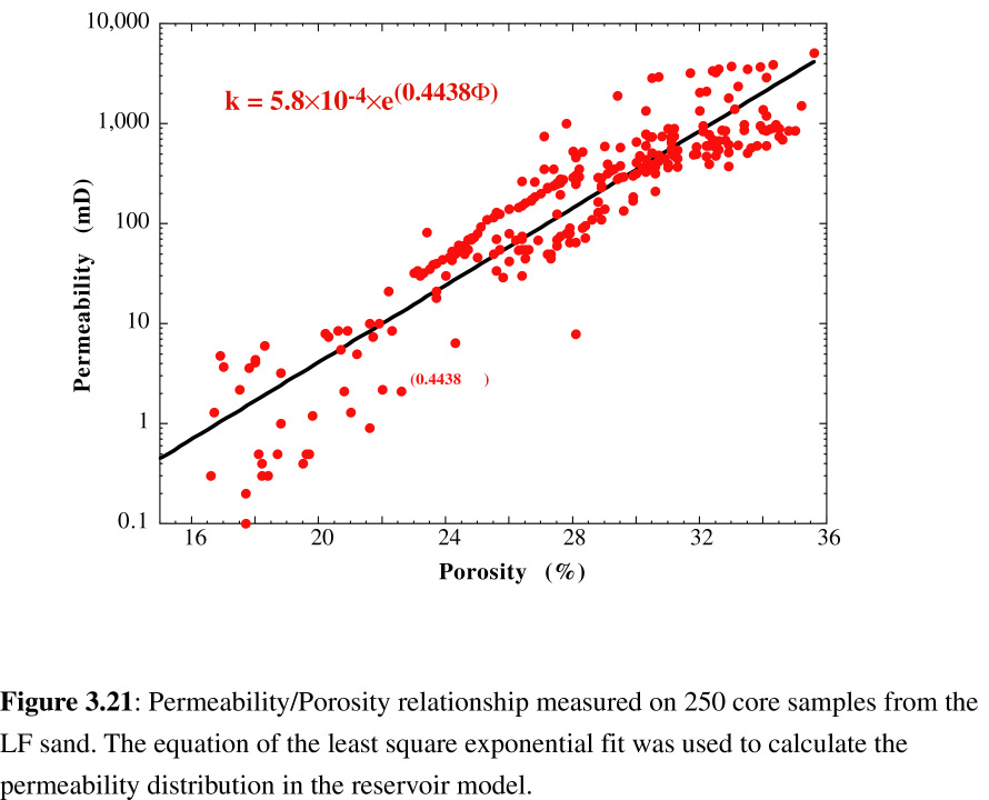
3.4.1 Permeability distribution
In addition to porosity, the primary control on the reservoir drainage is the permeability distribution. While permeability is directly related to porosity, it can also be affected considerably by the presence of shales [Audet, 1992, McCarthy, 1991]. In clean sands, permeability has been found to be an exponential function of porosity
 |
 |
| Figure 3.9 | Figure 3.10 |
The samples used were almost pure sandstone. McCarthy [1991] showed that the effects of porosity and shaliness (g) on the permeability of sand/shale mixtures are independent and that the effective permeability of shaly sandstones is:
3.4.2 Multiple-phase fluid flows in porous media
Reservoir simulation is based on solving the mass conservation equation of multiple-phase fluids in porous media, which can be expressed for a finite volume V within a surface A by:
The relative permeability of each phase increases with its saturation and can be calculated in three phases fluid as a combination of the relative permeabilities of two-phases fluid mixtures:
The code used to solve Eq (20) is ECLIPSE, a commercial three phase, three dimensional finite differences simulator using a corner point geometry grid that allows to define highly distorded nodes to represent the reservoir geometry [Ponting, 1989]. The position and the shape of each grid block is defined by the coordinates of its eight "corners". The coordinates and the attributes of the grid blocks (porosity and permeability) are directly imported from the reservoir characterization grid. The numerical formulation of Eq. (20) in finite differences for a grid block n connected to a number of blocks m is:
![]() (25)
(25)
Since the only actual measurable effects of the reservoir drainage are the volumes of hydrocarbons collected at the surface, the production history recorded on the rig floor is the principal constraint on the simulator. It is expressed in terms of daily production rate of oil or gas for each well, and averaged monthly. This imposed production is translated into pressure gradients between the wellbores and the formation, which are echoed in the reservoir at each time step of the simulation. The flow rate of phase j across an open wellbore interval is
ro = pressure equivalent radius of the grid block = 0.14 (Dx2 + Dy2)1/2
Mj = phase mobility = krj/mjBj
where Pj is the pressure of phase j in the node containing the connection, Pwell the pressure in the well at the depth of the connection, k the absolute permeability of the node, rw the well bore radius, S the skin factor representing the effect of formation damage, partial penetration or well deviation, Dx and Dy are the horizontal dimensions of the grid block and Bj is the formation volume factor of phase j, or its volumetric change from surface to reservoir conditions.
In addition to the perforated well intervals, the only flows allowed in and out the reservoir model are from eventual aquifers. The strength of the aquifer support is defined in water influx per unit pressure difference. All other model boundaries are considered impermeable, either lithologically (shaled out) or structurally (sealing faults).
By default, ECLIPSE uses a fully implicit solution procedure to solve Eq. (23), but in the case of regular grids and short time steps, the IMPES method (Implicit Pressure, Explicit Saturation) can be used for faster and less dispersive simulation but is more unstable than the default fully implicit formulation [Coats, 1992].
3.4.4.1 Constraint on the simulation: production history analysis
The production history imposed
on K8 during the simulation was the oil simulation shown in Figure
3.3a. A-12 was the only producing well from September 89 to June 1992.
The primary control of the success of the simulation was to reproduce the
gas production and pressure evolution histories (Figures
3.3b). The parallelism between oil and gas production before 1993 shows
that during this period reservoir pressure was above bubble point and reservoir
oil was undersaturated with a constant GOR. At the beginning of 1993 the
increase in gas production relative to oil production indicates that gas
started coming out of solution and that the reservoir pressure in the vicinity
of the wells was below the bubble point (51.7 MPa). This gas exsolution
is most likely responsible for the decrease in impedance observed between
the two seismic surveys in most of the upper layers of the reservoir and
updip from the wells .
| Figure 3.11 | 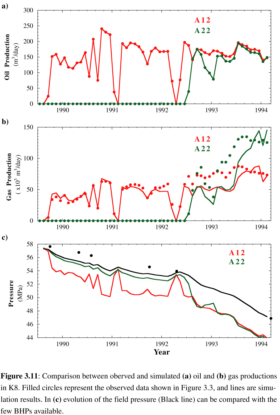 |
Figure 3.11 shows how the simulator
was able to reproduce the production history of K8, starting from the initial
conditions determined in 1988. Dots represent observed production data
(from Fig 3.3) and the lines the simulation results.
Because oil production was the imposed control mechanism, the perfect match
for this production was expected. The poorer match in gas production (Fig
3.11b) indicates that we were not able to reproduce the exact evolution
of K8, despite the good agreement of the simulated reservoir pressure (black
line in Fig 3.11c) with the few pressure measurements available (black
dots). The significant difference in the simulated pressures between the
average field pressure and the BHPs of the producing wells shows the artificial
pressure drawdown in the wells generated by intense production. The spikes
in the simulated A12 BHP correspond to short periods where this well was
shut down and the borehole started re-equilibrating with the surrounding
reservoir conditions.
 |
 |
| Figure 3.12 | Figure 3.13 |
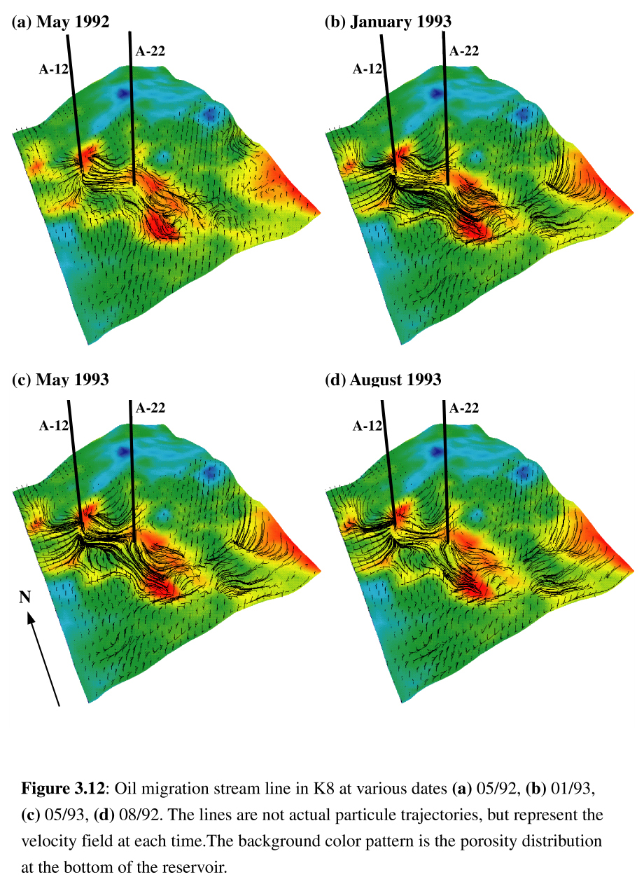
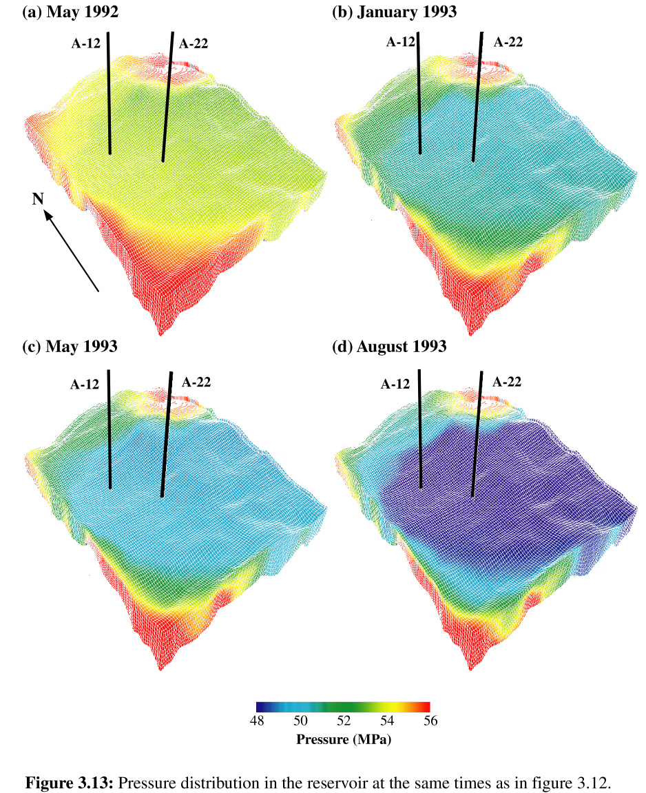
Even without matching the exact production history, the simulation helps to understand the dynamics in the reservoir. Figure 3.12 shows the simulated oil streamlines at various times in the simulation. In May 1992, A-12 is the only well producing, and all streamlines converge towards this well. In January 1993, shortly after the beginning of production in A22, some of the streamlines are heading for this well, but the main flow is still bypassing A22 downdip, towards A12. At the two later time steps, the streamlines become equally focussed on the two wells. As long as A12 was the only producing well, migrations occurred mostly in the center of the reservoir. The activation of A22 drove the oil in the western part of the reservoir to flow downdip (to the south) before heading west across the bulk of the reservoir towards the wells. This counter-buoyancy drive requires a consequent pressure drawdown in the south, confirmed by the evolution of the pressure field in Figure 3.13.
3.4.4.2.2 Fluid saturations
and impedance
 |
 |
| Figure 3.14 | Figure 3.15 |
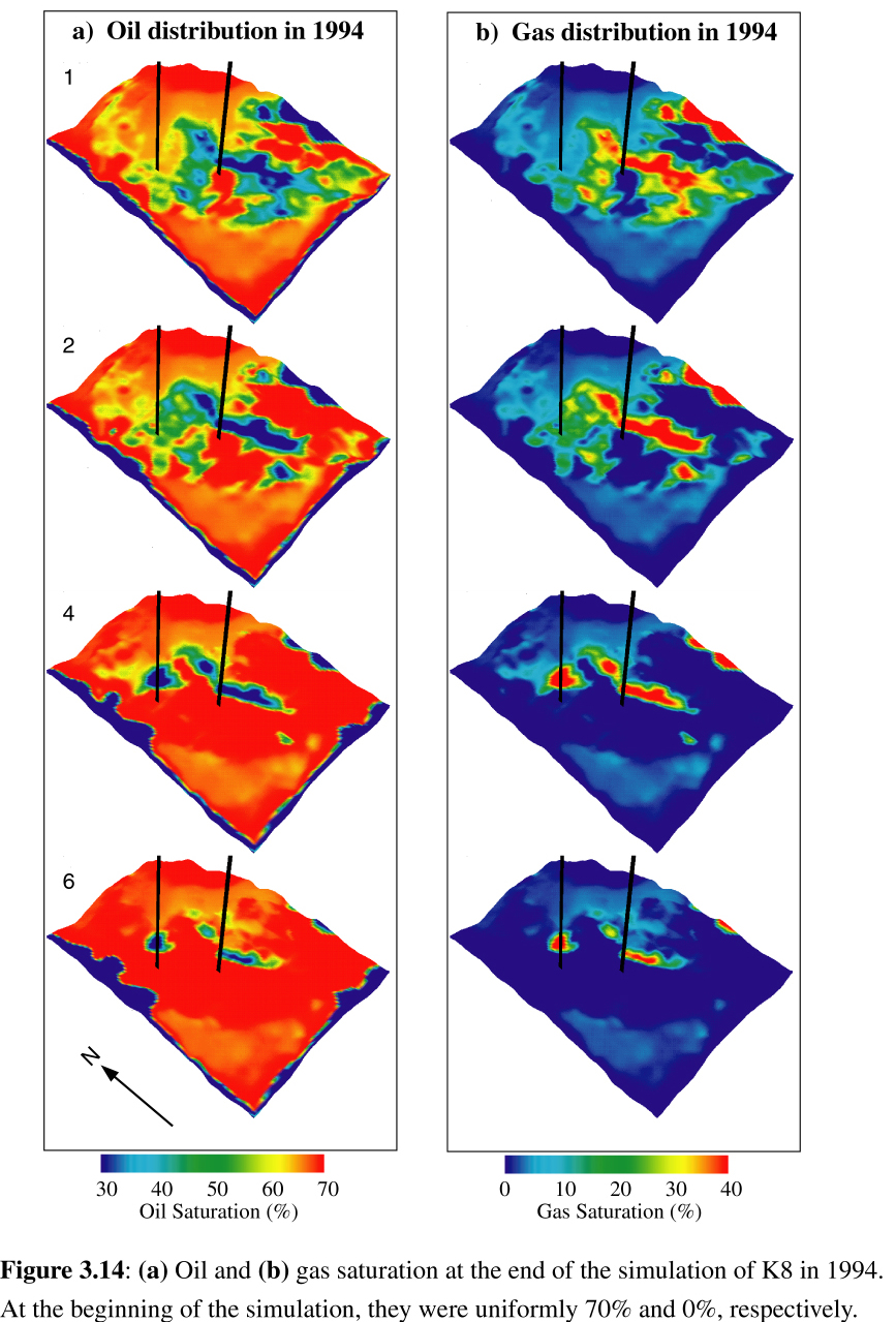
Figure 3.14 shows the oil and
gas distributions at the end of the simulation, which have to be compared
with the uniform values of 70% oil and no gas at the origin of the simulation.
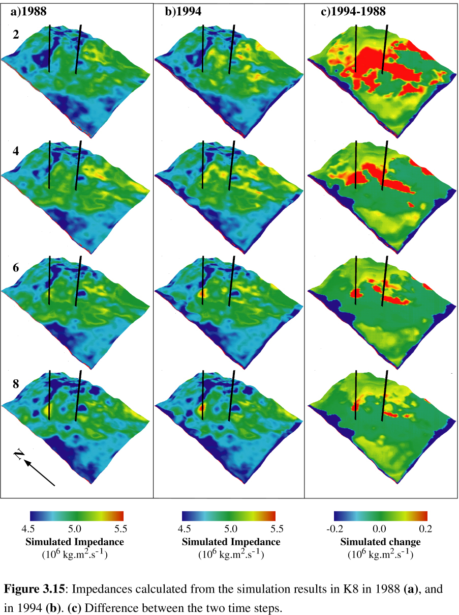
Figure 3.15 shows the impedance volumes and changes over time calculated
with these values using the Gassmann+Han formulation. The simulated impedance
distribution in 1994 (Figure 3.15b) seems very similar to the inversion
results at this date (Fig 3.4b), but to confirm that
this relationship still offers the best representation of the reservoir
properties after fluid substitutions, we also calculated the impedances
after the simulation with the other petrophysical formulations. Figure
3.16 shows the crossplots comparing the different model predictions to
the 1994 inversion. As before production, the KT and Gassmann+KT results
display the poorest agreement with the inverted impedance, showing even
a lower correlation in 1994 than at the origin of the simulation. Figs
3.16c and 3.16d confirm that the impedances calculated with Han and Gassmann+Han
still present the best comparison with the inverted impedance after fluid
substitutions. A crossplot between the two inversion results (Figure 3.16f)
shows that the regressions between the 1994 impedance and the Han and Gassmann+Han
models at this date are better than the comparison between the two impedance
volumes. This indicates that the errors in the elastic formulations are
lower than the changes that they are supposed to quantify, which is a prerequisite
for any meaningful quantification. As a step of the 4-D analysis loop,
similar comparison between various models should be performed for any reservoir,
because some formulations might be more appropriate for different depths,
pressures or lithologies. For the K8 sand, and for the LF330 reservoir
which has a very similar lithology, the combination of Gassmann/Hamilton
and Han were the most suitable.
| Figure 3.16 | 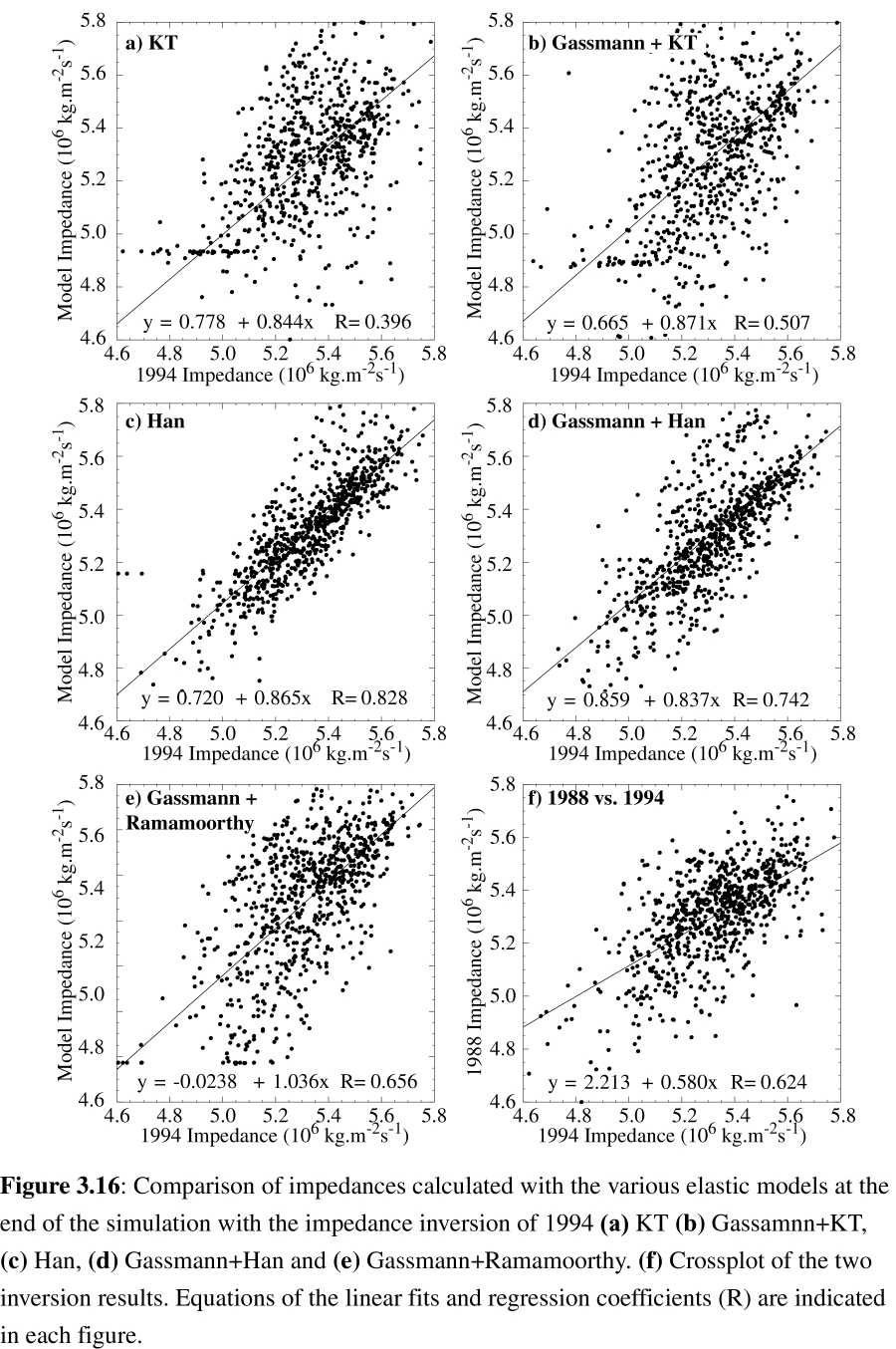 |
The comparison of the observed impedances changes over time (Figure 3.4c) with the simulated gas saturation and impedances changes (Figures 3.14b and 3.15c) confirms that the impedance decrease observed directly updip from the wells corresponds to an increase in gas saturation. The impedance decrease in the simulation results does not extend as broadly in the NE part of the reservoir as in the inversion differences. The decrease indicated by the inversions in this area can actually be caused by the production and the gas exsolution in the underlying K16 reservoir which merges with K8 at the crest of the structure. In the SW of the reservoir, downdip from the wells, the results of the simulation indicate a stronger decrease in impedance than observed from the inversion. This simulated decrease is generated by 10 to 15% free gas that came out of solution in this low-porosity part of the model (Fig 3.14b). This could show that the connectivity is higher in this area downdip from the bulk of the reservoir than in our reservoir characterization. Instead of remaining trapped in this corner most of the ex-solved gas should migrate updip to the wells. A higher gas relative permeability could also allow a more efficient mobilization of the gas. In any case, the considerable gas exsolution prevents the oil from being effectively drained in the deeper layers (Fig 3.14a), and a possible way to recover this oil would be to increase the pressure to re-dissolve the free gas. A program was initiated in 1997 for this purpose by injecting water downdip from the oil-water contact [Anderson et al., 1998]. To recover hydrocarbon which are bypassed in the migration shown in Fig 3.12, both simulation results and inversions indicate that the eastern flank of the reservoir could still contain large amounts of unproduced hydrocarbons.
3.5 LF sand, Eugene Island 330
The production history match is not perfect and the differences between simulated and inverted impedances changes show that our analysis of K8 needs refinement, but such discrepancies have to be expected when putting together so many types of data and disciplines in an integrated interpretation. Reducing or explaining the discrepancies is the object of the following steps of the 4D interpretation before spudding a new well.
The case of the LF reservoir, Eugene Island Block 330, is more complex, because of a much longer production history (more than 20 years), and more producing wells (14). It will underline the difficulties in time-lapse analysis and the need for an integrated multidisciplinary iterative loop to optimize the 4D interpretation.
3.5.1 Geological setting and history
The LF sand is one of the most
productive reservoirs in the Eugene Island 330 (EI330) field, the world's
most prolific Pleistocene oil field [Anderson et al., 1993], 200
km South-West of New Orleans (Figure 3.1). Because
of its exemplary longevity, EI330 has been one of the most thoroughly studied
fields in the Gulf of Mexico since its discovery in 1971. It has been the
object of multiple seismic surveys and provided a large amount of core
and log data, making it a typical case for petrophysical characterization
and time-lapse interpretation. The more than 25 sands that constitute the
field are stacked under rollover anticlines within an active growth fault
system. Down-to-the-basin and antithetic faults have divided the field
into several fault blocks, sealing laterally individual sand compartment
to form a total of more than 100 separate reservoirs [Holland, 1991].
The LF sand is a Pleistocene distributary-mouth bar deposit, thickening
progressively from the shaled out crest of the anticline on the East to
about 40 meters to the West. The top of the reservoir dips gently 10-20°
to the west, from 1900 mbsf at the crest to 2300 mbsf (Figure 3.17).
| Figure 3.17 | 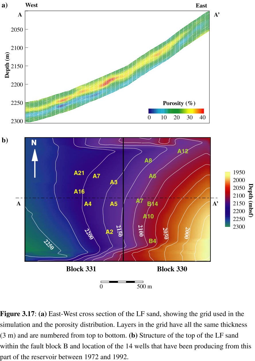 |
The 3 x 2 km study area is centered
on the boundary between Blocks 330 and 331 within the fault block B of
the Red Fault system [He, 1996]. In this compartment alone, 14 wells
have produced 2.75 million m3 of oil and 550 million m3
of gas since 1972. While production has been slowing down over the years,
the depletion rate has been particularly slow [Anderson et al, 1993],
and the four wells still producing after 1985 recovered 130,000 m3
of oil and 40 million m3 of gas between the two 3D surveys of
1985 and 1992 ( Figure 3.18)
| Figure 3.18 | 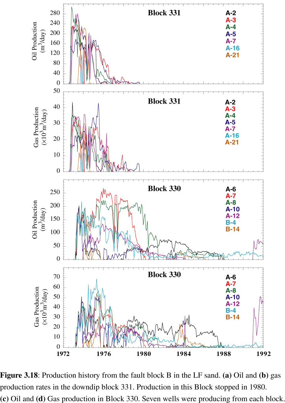 |
3.5.2 Preliminary 4-D impedance analysis
The results of the seismic impedance
inversions in 1985 and 1992 are shown in Figure 3.19. Because of its greater
quality, the 1992 survey was used as the base for the re-bining before
inversion, resulting in a spacing of 23 m along the dip direction, 15 m
along strike and 1.0 m vertically, for a total grid dimension of 134´
125´ 61 nodes.
In the two inversions, the lowest impedances are found in the bulk of the
reservoir (layer 24 in Fig 3.19), where the higher porosity reinforces
the influence of fluid distribution on the elastic properties.
| Figure 3.19 | 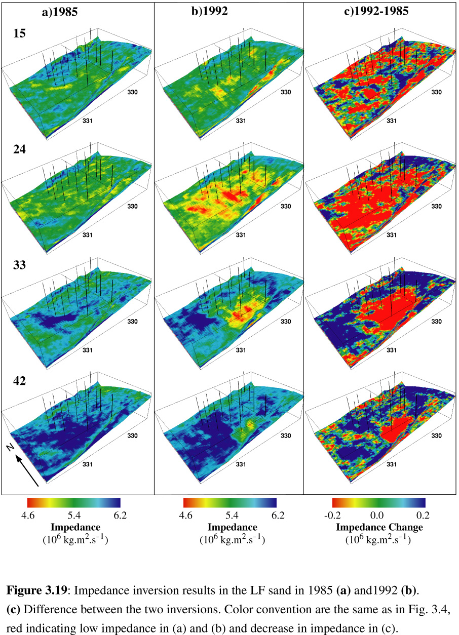 |
The subtraction of the two impedance volumes in figure 3.19c shows the changes that occurred during the seven years between the surveys. In the upper layers, impedance has decreased almost uniformly, likely because of continuous pressure decrease and gas exsolution. In the deeper layers, impedance generally increased as water was replacing oil, except in two locations: on the northern edge of Block 330, where A-12 was re-activated in 1991 to produce mostly gas and where A-6 and A-8 were active until 1988, and in a large area centered on the block line downdip from well B4, which was the most productive well during this period. The lateral extent of this "brighter" area decreases with depth, but it extends surprisingly far downdip in Block 331, where no well was active between the two surveys.
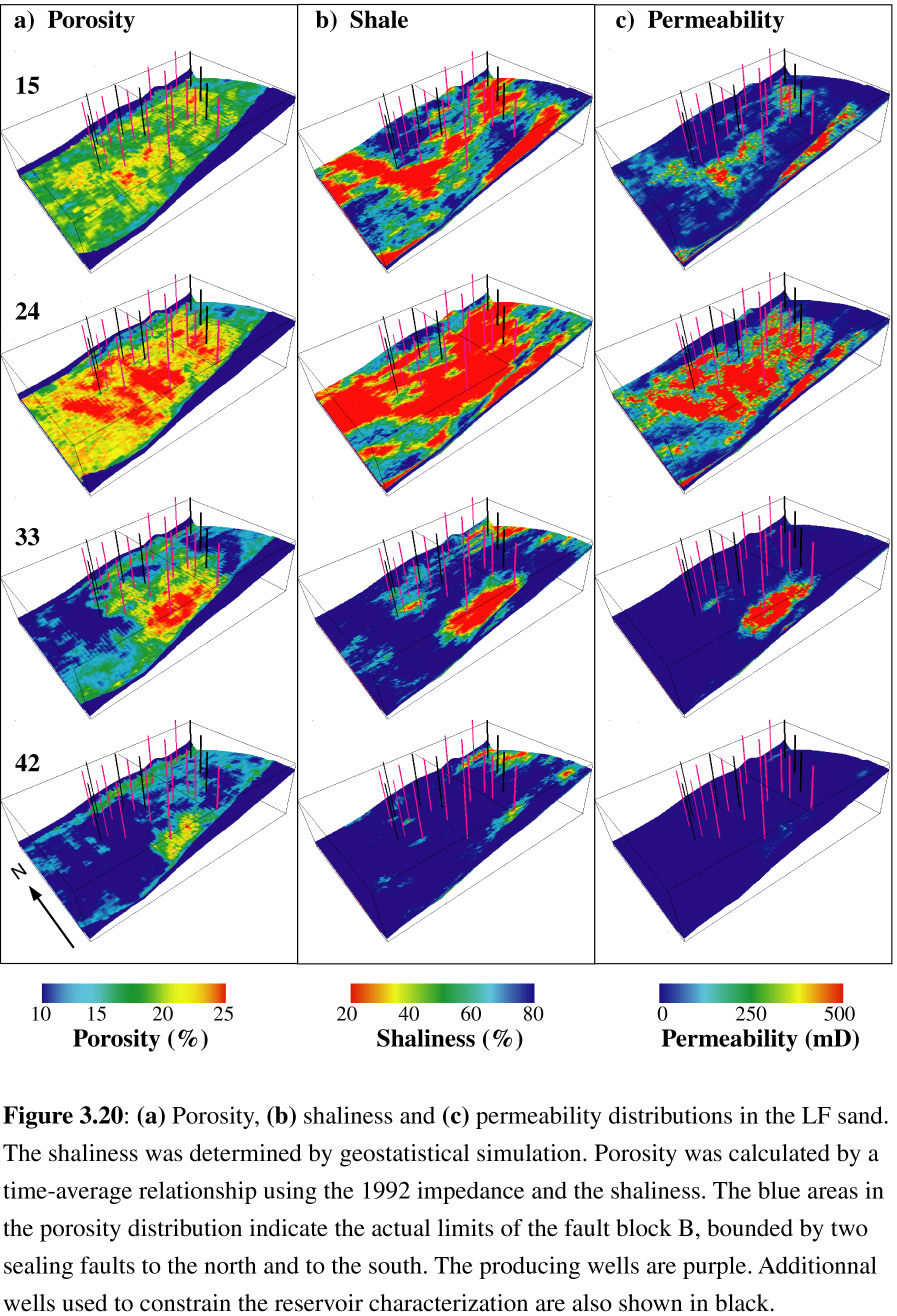
3.5.3 Reservoir characterization of LF330
He [1996] used GR and SP
logs from 20 wells to calibrate the geostatistical characterization of
the lithology, using the 1992 impedance volume as soft data. Because only
a few porosity logs were available in Block 330, it was not possible to
use an independent geostatistical simulation to determine porosity distribution.
Instead, porosity was calculated with the time average relationship (Eq.
17) and the results of the lithology characterization. The resulting lithology
and porosity distributions are shown in Figure 3.20. Because of the absence
of log-derived correlation functions, the porosity distribution inherits
the low spatial correlation of the impedance volume, which prevents from
identifying eventual high porosity channels and results in a porosity generally
lower than the actual reservoir values (see porosity values of clean samples
in Fig 3.21). Permeability measurements on 250 core samples (Fig 3.21)
were used to establish the permeability-porosity relationship in the LF
sand. The effective permeability distribution (Figure 3.20c) was calculated
with an exponent m = 2 for the shale fraction in Eq. (19).
 |
 |
| Figure 3.20 | Figure 3.21 |
The resolution of the impedance volume was upscaled by 3 in the reservoir simulator, resulting in a grid of 33´ 33´ 20 = 21780 nodes, with dimensions 69 m ´ 45 m ´ 3 m. In the upscaling process, both porosity and shaliness were calculated by volumetric average, and the permeability of each node in the model was calculated with the averaged attributes in Eq. (19).
3.5.4 Fluid properties and initial conditions
Because at the time of the first 3D survey (1985), the reservoir had already been producing for 13 years from 14 wells, the distribution of the fluids in place was too complex to assume proper initial conditions for the reservoir simulation at this time. Eventhough the period of interest was within the last seven years, it was necessary to start the simulation from the only fluid distribution that could be determined reliably, which was the hydrostatic equilibrium before production. The OWC and GOC were identified in 1972 at 2320 m and 2050 m respectively [Holland, 1991]. The location of the GOC at the crest of the anticline indicates that the upper part of the reservoir was at bubble point pressure (28.5 MPa) before the beginning of production. The other PVT parameters measured on LF hydrocarbon samples and used to calculate reservoir fluid properties are in Table 2. From these data we integrated the initial pressure and fluid distribution in 1972 in the same manner as for K8.
The results of the production
and pressure history match in blocks 331 and 330 are shown in Fig 3.22.
In block 331 (Figs 3.22a and 3.22b), where most wells produced only until
1977, the simulated productions (lines) match almost perfectly the recorded
data (diamonds). The good oil production match was forced as the engine
of the simulation. Because of the greater depth in this part of the reservoir
and of its short production activity, the pressure remained close to bubble
point in most of Block 331 during its producing history. Consequently,
gas saturation never exceeded the critical gas saturation value and gas
production remained almost proportional to the oil production with constant
GOR. The most significant mismatches in block 331 occur with wells A3 and
A5, where the simulation does not reproduce the gas production increases
observed in 1975. This increase indicates that at this time the gas cap
must have reached A3 and A5, the most updip producing wells of Block 331.
The simulation is therefore lagging reality in the extension of the gas
cap. However, the good reproduction of the pressure evolution in the field
(Fig 3.22e) shows that the mismatch could be related to errors in connectivity
in the vicinity of the wells, while the reservoir is behaving properly
overall.
| Figure 3.22 | 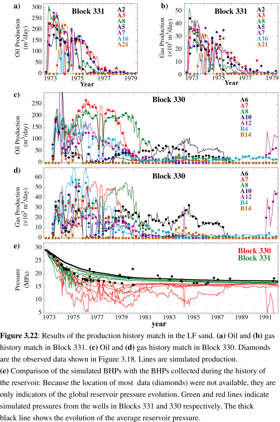 |
In Block 330 (Figs 3.22c and 3.22d),
the presence of the gas cap at the onset of production makes the relative
productions of oil and gas depend intimately on the correct evolutions
of the local pressure fields and of the saturations of the different phases
which controls the relative pemeabilities. Volumes of oil produced are
usually more accurately recorded than gas production, and are consequently
more reliable constraints for the reservoir simulation. However, we were
able to get a better cumulative oil and gas match by forcing gas production
instead of oil in two wells: A-12 and A-6. Forcing oil production in these
wells resulted in gas production much lower than observed, the oil and
gas production remaining proportional to each other. This could show that
porosity, and permeability, are lower in the vicinity of these wells than
estimated from our time-average relationship. With lower formation permeabilities,
the pressure gradients required to produce the same amount of hydrocarbon
would be higher, generating lower pressures around the wells, and therefore
higher produced gas/oil ratio. The uncertainty in the porosity estimation
is a direct consequence of the lack of reliable well data in the northern
part of Block 330 where A-6 and A8 are located [He, 1996]. However,
the good reproduction of the pressure evolution (Fig 3.22e) and the overall
good match of the most of the wells production suggest that we reproduced
reasonably well the volumes of the different phase migrations. In particular,
the very good match for Block 331 and the good match in Block 330 in the
first years of the simulation indicate that the conditions in the field
at the time of the first survey should be similar to the results of our
simulation in 1985.
 |
 |
| Figure 3.23 | Figure3.24 |
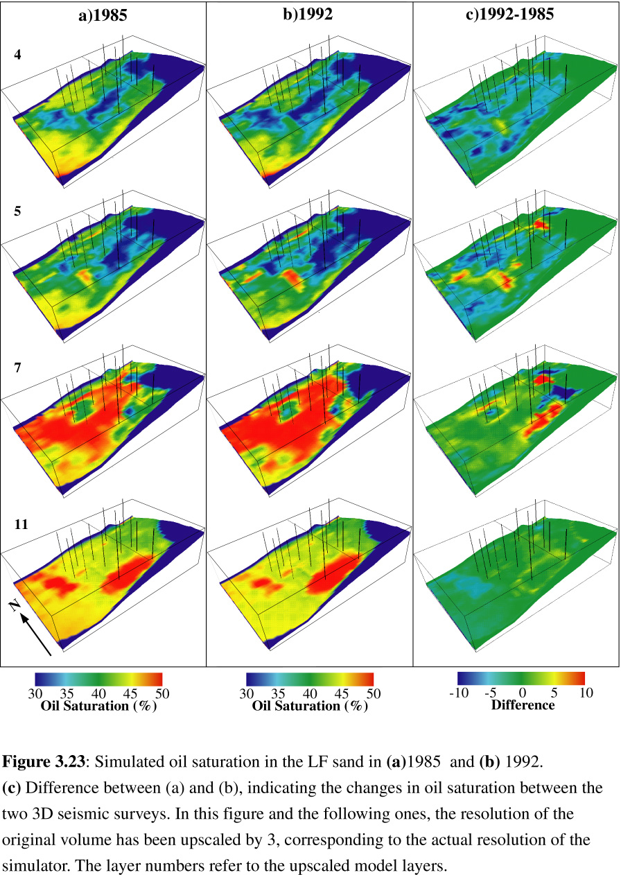
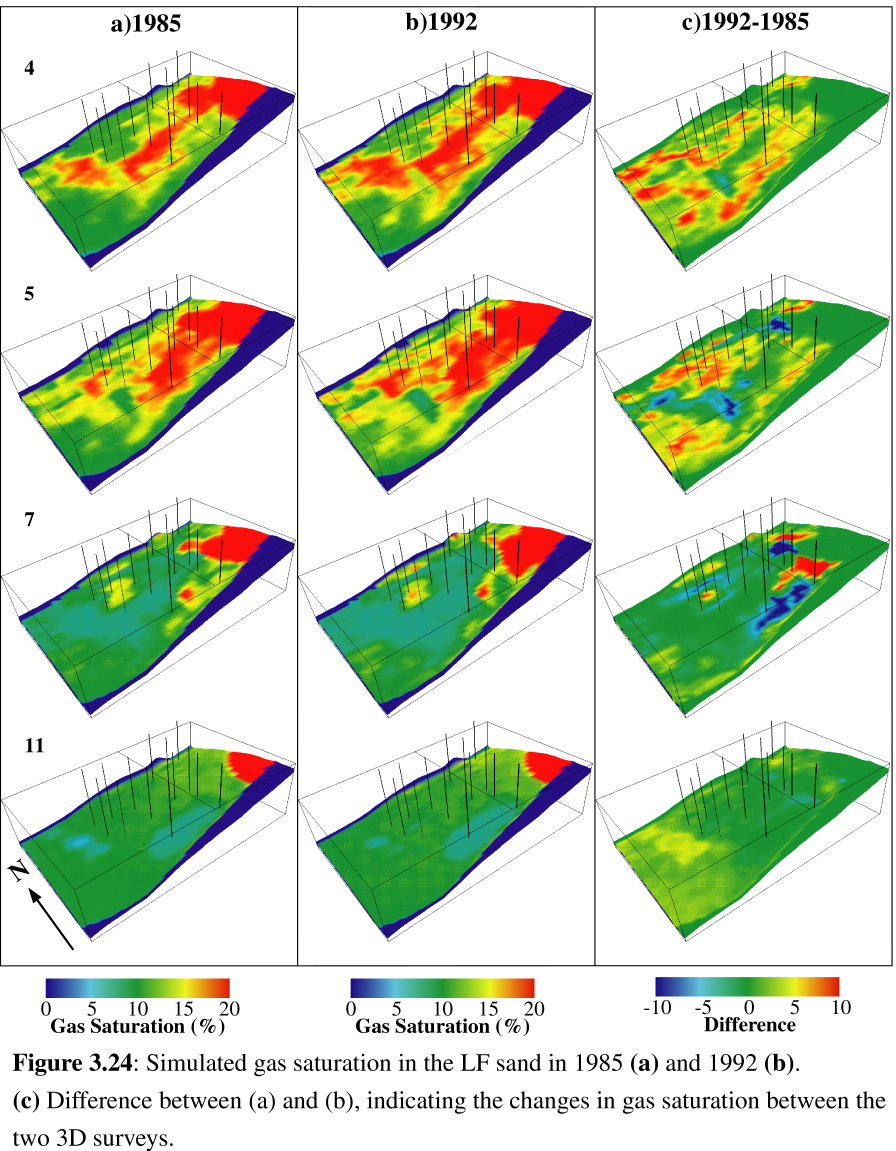
The results of the simulation
in terms of oil and gas saturations at the time of the two surveys are
shown in Figure 3.23 and 3.24. The comparison of gas saturation and inverted
impedance changes shows that the impedance decrease observed in the shallower
part of the reservoir between the two surveys can be associated with an
increase in gas saturation. Figure 3.24c shows that, despite the absence
of production activity in Block 331 between the two surveys, the gas cap
kept extending downdip in this block, confirming our preliminary impedance
interpretation. However, this qualitative association between gas increase
and impedance decrease does not translate quantitatively in the impedance
distribution and impedance changes calculated from the simulation results
(Fig 3.25).
| Figure 3.25 | 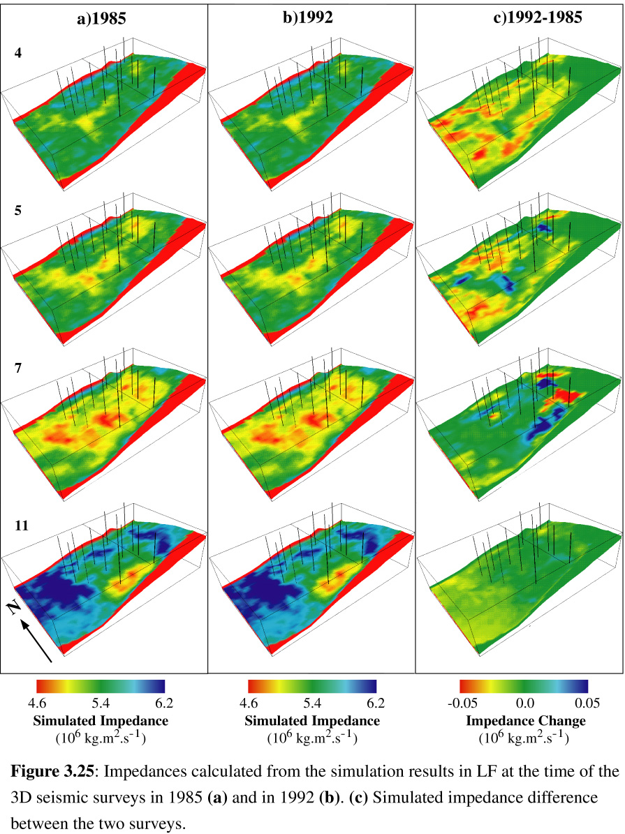 |
Both impedance volumes calculated in 1985 and 1992 appear generally similar to the inversion results, but the discrepancies between simulation and inversion are apparent when comparing the simulated and inverted impedance changes over time (Fig 3.19c vs. 3.25c). By removing most of the contribution of the matrix materials to the impedance, the differentiation between successive results is much more sensitive to possible disagreements between simulation and inversion. In particular, while the inversion results indicate a decrease in impedance at all depths in the central part of the reservoir (Fig 3.19c), this decrease is limited to the upper layers and the deeper layers in the simulation, where porosity and permeability are low and free gas coming out of solution remains trapped. In the bulk of the reservoir (see layer 8), the simulation results show an increase in impedance associated with oil replacing some of the free gas. Because of the relatively low production between the two surveys, the pressure decrease generated by production is balanced by the return to normal pressure in the reservoir after years of intense production. Figure 3.22e shows that between 1985 and 1992, the average field pressure decreased only slightly, while BHPs across the field increased after having been drown to values much lower than formation pressures. Although the impedance decrease interpreted from the inversion results at the center of the reservoir is clearly identifiable in Fig 3.19c, its amplitude is difficult to explain with only one well producing in the area (B4) at a rather sow rate (about 25 m3/day). Such inconsistencies between seismic inversion, reservoir simulation and actual production data are at the core of the 4-D optimization loop.
3.6 Discussion - End of the 4D loop
3.6.1 Discussion of the LF sand results
Some of imperfections of the LF simulation have to be attributed to the simplified porosity determination. A close look at the two survey times indicates that the agreement between inversion and simulation is better in 1992 than in 1985. This is due to the fact that the porosity distribution was explicitly derived from the 1992 inversion by a simple time average formulation. A qualitative comparison of the 1992 impedance inversion (Fig 3.19b) with the porosity distribution (Fig 3.20a) shows that the porosity pattern can be directly mapped on the 1992 impedance. Such direct relationship between reservoir characteristics and seismic attributes introduces a clear bias in the ability of the simulation to provide an independent validation of the 4D interpretation. For comparison, the porosity distribution in K8 (Fig 3.6a), which was calculated by a complete log-constrained stochastic characterization, cannot be directly mapped on any of the two impedance inversions (Fig 3.4).
Independently from this clear bias in the 1992 impedance match, the poor reproduction of the impedance changes in the LF sand underline the difficulties of time-lapse analysis. The only actual constraints on the progress of the simulation are the well production histories and the few pressures recorded, which are very localized data. It is therefore crucial to have reliable inversion results and a complete stochastic reservoir characterization for a precise volumetric reference at the time of the surveys. In the case of the LF sand, because the 1985 survey was acquired a time when 3D seismics were still in their infancy, it does not provide such dependable reference. The original time-lapse analysis of the LF sand was performed through the comparison of region-grown volumes [He, 1996]. This technique allowed the identification of migration patterns and a preliminary interpretation of the reservoir dynamics but can not be used for a quantitative estimation of the changes in the reservoir fluids distribution. The subtraction of the two impedance volumes that we use for our qualitative evaluation is much more sensitive than region-growing algorithms to the effects of differences in the acquisition of the two surveys. The low level of confidence in the 1985 impedance added to the inability to constrain the stochastic porosity simulation and to the recurrent absence of parameters such as relative permeabilities make the problem become clearly under-determined in this reservoir.
3.6.2 Closing the 4D analysis loop - optimization
Improving the present results and, more generally, the optimization of the 4D interpretation loop can take several forms. Different sources of uncertainty have been identified, in particular: (1) various numerical parameters and missing reservoir properties, (2) the numerical formulation of reservoir petrophysical properties and (3) results from steps preceding the reservoir simulation, such as seismic inversion and reservoir characterization.
Recurrently missing properties and numerical parameters such as relative permeability functions, critical saturations, capillary pressures, aquifer strength or the shale exponent in the effective permeability calculation can be varied between successive simulations in order to find a better history match. Upscaling the reservoir model dimensions for shorter computation times, it is possible to automate the variation of some of these arbitrary numerical parameters or loosely constrained properties to minimize the difference between measured and simulated production history.
The choice of the most representative petrophysical formulation (Han, Gassmann, KT or others) is crucial to establish the correspondence between impedance inversion and fluids in place. In addition to the formulation themselves, the elastic parameters of the grain matrix in these formulations can be varied to represent different lithologies and grain arrangements. The simple comparison between various formulations such as the crossplots used for K8 (Figures 3.7 and 3.16) can be improved by iteratively varying grain elastic parameters in order to improve the regressions. The relatively limited number of parameters in these formulations can allow simple automated optimization routines to identify the most appropriate model and the proper matrix properties.
Limiting the optimization to the identification of these parameters or to the choice of the petrophysical representation requires that more fundamental components of the 4D interpretation are dependable, in particular the impedance inversions and the reservoir characterization. Reservoir simulation can be used either to validate these prior results, or to constrain their re-evaluation. In the case of LF330, a major source of inaccuracy is the porosity distribution. In the absence of additional logs, a possible way to improve the porosity distribution is to use the simulation results to re-estimate the porosity from the 1992 inversion with the time-average relationship (Eq. 17) and the fluid distribution resulting from the simulation [He et al., 1998]. For all the imprecisions still resulting from the absence of stochastic parametrization and from possible errors in the simulation, the porosity calculated with these simulated saturations should be more appropriate than the uniform average "brine impedance" originally used. This procedure can be used more generally when no survey was shot before production and no reference survey with known hydrostatic fluid distribution provides a reliable reference such as in K8. This would provide a more accurate "soft" porosity distribution for the reservoir characterization.
In addition to the uncertainties in porosity distribution, the analysis of the LF sand is also impaired by the limited confidence in the 1985 seismic dataset. While the steady improvement of 3D acquisition techniques over the last few years has greatly reduced this source of concern for recently acquired datasets, it remains a primordial issue when using legacy datasets which were not acquired along the rigorous guidelines required by time-lapse seismic. The assessment of this uncertainty and of possible remedies requires to go beyond the parameters directly associated with the reservoir simulation. It requires to complete the 4-D analysis by returning to the initial steps of the interpretation loop and to the original data: seismic amplitude volumes.
To complete the loop, the impedance volumes calculated from the results of the reservoir simulation have to be fed into a 3D seismic waves propagation elastic model to try to reproduce the observed datasets. For this purpose, we have built tools allowing to remesh the simulation grid within the original data volume [Mello et al., 1998] and developed a full elastic 3D finite difference model to simulate the propagation of seismic waves and generate a synthetic seismic amplitude volume. The comparison of the simulated amplitudes with the original datasets can be used as a simple validation of the reservoir simulation, but it can also be used to re-evaluate the inversion or the reservoir characterization results when data are missing or unreliable. In the case of the LF sand, the impedance changes calculated from the reservoir simulation are much smaller than indicated by the subtraction of the two inversions. The reservoir simulation and the impedances calculated from its results might be only partially accurate, but since the simulated production volumes and pressure variations were equivalent to the actual production data, the range of the simulated impedance changes should be representative of the actual changes between the two surveys. If we assume that the 1992 inversion is the most accurate, this shows that the 1985 inversion has to be re-estimated. This can be done by applying the 3D elastic model to the 1985 simulated impedances. If the resulting seismic amplitudes volume compares well with the original 3D survey, the simulated impedances can be used as a new a priori impedance distribution for the re-evaluation of the inversion of the 1985 survey. Because most of the production occurred before the first 3D survey, the few wells producing after 1985 have merely been developing features of the earlier production phase. Therefore, properly simulating the reservoir before 1985 is as crucial to our time-lapse analysis as the simulation between the two surveys. This can only be completed by a good agreement between seismic inversion, reservoir simulation and elastic simulation at the time of this first survey.
These are mere possibilities for the 4D interpretation to proceed from reservoir simulation to get an exact understanding of the reservoir dynamics. Because the exploration, production history and the configuration of each reservoir are unique, there is no exhaustive procedure for time-lapse monitoring. We have tried to develop an integrated series of tools allowing to apply our general methodology to any reservoir, but its flexibility requires a clear understanding of the possible sources of errors in order to use the iterative procedure to minimize them.
At the junction between complex theoretical methods (non-linear seismic inversion, 3D elastic modelling or stochastic simulation) and the most primary field data, reservoir simulation provides the link between the observed changes in seismic attributes, the hydrocarbons produced on the rig floor and the actual fluid dynamics within a reservoir. Because it should ultimately indicate where to drill to recover trapped hydrocarbon, and the volumes to expect, it can help understand the passed history of a reservoir, but more importantly, how to make the best of its future. In the case of the K8 sand, the good agreement between simulation and inversion indicate that the final optimization should be only a refinement of the present results. Because of its more complex history and of the lesser quality of the available data, the complete assessment of the future of the LF sand requires a more profound overhaul of our original assumptions.
Completing our conclusions of chapters 1 and 2, we have shown how different types of elastic formulations can be used to quantify transformations of the pore space and of the pore materials in marine sediments. In the case of silica diagenesis and gas hydrate formation, these models allowed to describe the nature of the transformation of the pore space and understand very distinct seismic signatures of long-range processes. Their application to fluid substitutions in a producing reservoir can have direct short term implications: the spudding of a new well. In the last chapter, we describe how temperature and heat flow measurements can be used to identify the long term migrations in active fault zones feeding the LF sand and similar reservoir as we exploit them.
Anderson, R.N., G. Guerin, W. He, A. Boulanger and U. Mello, 4-D, 1998, Seismic reservoir simulation in a South Timbalier 295 turbidite reservoir, The Leading Edge, 17(10),1416-1418.
Batzle, M., and Z. Wang, 1992, Seismic properties of pore fluids, Geophysics, 57(11):1396-1408.
Beggs, H.D., 1992, Oil system correlations, in Petroleum Engineering Handbook, Bradley, Ed, Third printing, part 22, SPE, Richardson, TX.
Coats, K.H., 1992, Reservoir Simulation, in Petroleum Engineering Handbook, Bradley, Ed, Third printing, part 48, SPE, Richardson, TX.
England, W.A., A.S. Mackenzie, D.M. Mann and T.M. Quigley, 1987, The movement and entrapment of petroleum fluids in the subsurface, J. of the Geol. Soc., London, 144, 327-347.
Gassmann, F., 1951, Elastic waves through a packing of spheres, Geophysics, 16, 673-685.
Guerin, G., and D. Goldberg, 1996, Acoustic and elastic properties of calcareous sediments across a siliceous diagenetic front on the eastern U.S. continental slope, Geophys. Res. Lett., 23(19), 2697-2700.
He, W., 1996, 4-D Seismic Analysis and Geopressure Prediction in the Offshore Louisiana, Gulf of Mexico. Ph.D. Thesis, Columbia University.
He, W, G. Guerin, R.N. Anderson, and U.T. Mello, 1998, Time-dependent reservoir characterization of the LF sand in the South Eugene Island 330 Field, Gulf of Mexico, The Leading Edge, 17(10).
Hamilton, E.L., 1971, Elastic properties of marine sediments, J. Geophys. Res., 76, 579-601.
Hamilton, E.L., Bachman, R. T., Berger, W. H., Johnson, T. C., and Mayer, L. A., 1982, Acoustic and related properties of Calcareous deep-sea sediments, J. Sed. Pet., 52(3), 733-753.
Han, D-H., A. Nur and D. Morgan, 1986, Effects of porosity and clay content on wave velocities in sandstones, Geophysics, 51(11), 2093-2107.
He, W., Holland, D. S., Leedy, J. B., and Lammlein, D. R., 1990, Eugene Island Block 330 field-U.S.A., offshore Louisian, in Beaumont, E.A., and Foster, N. H., compilers, Structural traps III, tectonic fold and fault traps: AAPG Treatise of Petroleum Geology Atlas of Oil and Gas Fields: 103-143.
Hoover, A.,1997 Reservoir and production characteristics of the South Timbalier 295 field, offshore Louisiana, with comparison to outcrop analogue and 4-D seismic results, M.S. Thesis, Pennsylvania state university.
Kuster, G.T., and M.N. Toksöz, 1974, Velocity and attenuation of seismic waves in two-phase media, 1, Theoretical formulation, Geophysics, 39, 587-606.
Mason, E.P., 1992, Reservoir geology and production performance of turbidite sands at South Timbalier 295 field, offshore Louisiana, in transactions of the Gulf Coast Association of Geological Societies, Vol XLII, 267-278.
McCarthy, J.F., 1991, Analytical models of the effective permeability of sand-shale reservoirs, Geophys. J. Int., 105, 513-527.
Mello, U.T., P.R. Cavalcanti, A. Moraes and A. Bender, 1998, New developments in the 3D simulation of evolving petroleum systems with complex geological structures, AAPG international conference and exhibition abstracts, AAPG Bulletin, 82(10), p. 1942.
More, J., 1977, The Levenberg-Marquardt algorithm, implementation and theory: numerical analysis, G.A. Watson, Ed., Lecture notes in Mathematics, 630, Springer-Verlag.
Murphy, W.F, A. Reischer, A., and K. Hsu, 1993, Modulus decomposition of compressional and shear velocities in sand bodies, Geophysics, 58(2), 227-239.
Ponting, D.K., 1989, Corner Point Geometry in Reservoir Simulation, proc. Joint IMA/SPE European Conference on the Mathematics of Oil Recovery, Cambridge.
Ramamoorthy, R., W.F. Murphy and C. Croll, 1995, Total porosity estimation in shaly sands from shear modulus, Trans. SPWLA 36th Logging Symposium, paper H.
Rose, W., 1992, Relative Permeability, in Petroleum Engineering Handbook, Bradley, Ed, Third printing, part 28, SPE, Richardson, TX.
Steffensen, R.J., 1992, Solution-Gas-Drive reservoirs, in Petroleum Engineering Handbook, Bradley, Ed, Third printing, part 37, SPE, Richardson, TX.
Tucker, B., 1997, Time-lapse seismic monitoring of the South Timbalier Block 295 field, offshore Louisiana, M.S. Thesis, Pennsylvania state university.
Tosaya, M.N., and A. Nur, 1982, Effects of diagenesis and clays on compressional velocities in rocks, Geophys. res. lett., 9, 5-8.
Zimmerman, R.W., and M.S. King, 1986, The effect of the extent of freezing on seismic velocities in unconsolidated permafrost, Geophysics, 51, 1285-1290.
|
|
|
|
|
|
|
|
|
|
|
|
|
|
|
|
|
|
|
|
|
Table 2 : Properties of the reservoir fluids used in the simulation and in the elastic models
|
|
|
|
|
|
|
|
|
|
|
|
|
|
|
|
|
|
|
|
|
|
|
|
|
|
|
|
|
|
|
|
|
|
|
|
|
|
|
|
Appendix: Reservoir fluids properties
In an ideal time lapse analysis, a complete PVT analsis of reservoir fluid samples should provide the exact relationships between reservoir fluid properties, pressure and saturation. The main parameters required for the simulation and for calculating impedances are mostly compressibility, density, viscosity. In a typical case only some of these relationships are actually measured, and only a few parameters are systematicaly measured. Batzle and Wang [1992] provide a very complete description of the elastic properties of reservoir fluids. We summarize here the few relationships that can be readily used in a typical 4D analys using only the few parameters that are systematically measured: the oil and gas gravities, reservoir temperature and pressure. In all the following relationships, Temperature is in ° C, Pressure in MPa, density in g.cc-1 and bulk modulus in MPa.
Brine properties:
In most reservoirs, brine samples are analysed for such purposes as logs calibration or reservoir evaluation. In the absence of brine samples, a linear fit to the data compiled by Batzle and Wang [1992] provides a way to estimate salinity (S) vs. depth (z, in m):
The density of water rw can be approximated by a polynomial function of pressure and temperature:
rbrine = rw + S[0.668 + 0.44S + 10-6(300P - 2400PS + T(80 + 3T - 3300S - 13P + 47PS))] (24)
|
|
|
|
|
|
|
|
|
|
|
|
|
|
|
|
|
|
|
|
|
|
|
|
|
|
|
|
|
|
|
|
|
|
|
Gas properties:
Gas mixture properties can characterized by their specific gravity, G, which is the ratio of the gas density to air density at standard conditions.
For temperatures and pressures typically encountered in oil fields, the gas density (rg) and bulk modulus (Kg) can be calculated by:
 (27)
(27)
with ![]() (29)
(29)
![]() and
and ![]() .
(30)
.
(30)
and ![]() (31)
(31)
Oil properties
The properties of oil vary differently wether pressure is higher or lower than the bubble point. In any case, if PVT analysis results are not availbable, elastic properties can be calculated from its density roat standard surface condition, the gas gravity G and the bubble point pressure. Oil gravity is usually expressed by its American Petroleum Institute (API) gravity:
![]() (34)
(34)
Below bubble point, the `oil' phase is saturated with dissolved gas and its composition varies as pressure decreases and more light hydrocarbon come out of solution. The density of this `live' oil is given by:
![]() (35)
(35)
where RG = 2.03[Pe(0.02878API - 0.00377T)]1.205 (36)
and ![]() (37)
(37)
The velocity can be calculated by replacing ro in (33) with a pseudo density r' representing the expansion caused by gas intake:
in both cases, the bulk modulus is calculated from density and velocity by
![]()
