Making Pseudoproxies

Making Pseudoproxies
Friday, March 11, 2011
Once climatic series (in this case temperature) are sampled from given locations in the model field for pseudoproxy experiments, researchers have to decide how to add noise to these series to mimic the noise contained in real proxy data. If noise is not added, the sampled temperature time series are perfect “measurements” of local temperature in the model field, which could never be the case in the real world. Real climatic proxy records (e.g. trees rings, ice cores, cave deposits, coral skeletons, etc.) process climatic variations through their own multivariate and non-linear filters. This process of filtering obscures the climate signals contained in real-world proxy records by combining them with non-climatic noise. To mimic these processes in pseudoproxy experiments, noise is added to the locally sampled temperature series. There are many ways in which this noise can be introduced. The simplest approach is to add different amplitudes of white, i.e. Gaussian, noise to the temperature time series. While the noise in real-world proxies is almost certainly not white, we can think of experiments using white noise as a baseline representing the best-case scenario for how our reconstruction methods might perform.
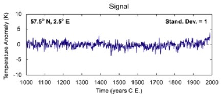
To demonstrate the addition of white noise to a temperature time series, consider the one shown at the top of this post. Now consider a white noise time series that is scaled as follows: (1) its standard deviation is equal to the temperature time series; (2) its standard deviation is twice that of the temperature time series; and (3) its standard deviation is four times that of the temperature time series. These white noise time series are shown below and are plotted on axes with the same scaling as above. The correlation with the temperature time series is also given in the plot (and is very low as expected).
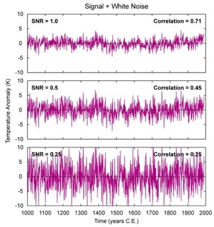
Now imagine adding each of the white noise series above to the original temperature time series. The result is shown in the above figure on the right. These combined time series can be thought of as having both a temperature signal and noise in proportions that are characterized by the Signal-to-Noise Ratio (SNR). For the three cases above, the SNRs are 1, 0.5, and 0.25, by standard deviation. The correlations between the combined time series and the original temperature time series are also shown in the plot. As expected, these correlations reduce as the amplitude of the noise increases and the SNR becomes smaller.
The above example illustrates how real-world proxy data are interpreted as being a combination of signal and noise (albeit with more complicated noise characteristics). In pseudoproxy experiments, such combined signal and noise series become the pseudoproxies that we use to test reconstruction methodologies. We’ll show more about how this is done in following posts.
***Update (2/2/2012): Please note my review on pseudoproxy experiments published in WIRES Climate Change:
Smerdon, J.E. (2012), Climate models as a test bed for climate reconstruction methods: pseudoproxy experiments, WIREs Clim. Change, 3:63-77, doi:10.1002/wcc.149.
A single annual temperature time series sampled from the ECHO-g millennial simulation.
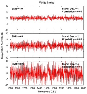
White noise time series scaled to have standard deviations 1, 2 and 4 times the standard deviation of the temperature time series shown at the top of this post.
Time series created by combining the white noise in the figure on the left with the temperature time series plotted at the beginning of this post. Correlations given in the plots are between the combined time series in the figure and the original temperature time series.

