Pseudoproxy Experiments

Pseudoproxy Experiments
Friday, March 11, 2011
An important new tool for evaluating the performance of climate reconstruction techniques has come to be known as pseudoproxy experiments (Mann and Rutherford, 2002), which use millennial simulations from General Circulation Models (GCMs; González-Rouco et al. 2003, 2006; Ammann et al. 2007) as the basis of synthetic experiments. The idea behind the pseudoproxy approach is to use a simulated model climate as a test bed on which to evaluate the performance of a given reconstruction method using controlled and systematic experiments. Although one must always be mindful of how pseudoproxy results translate into real-world implications, the flexible design capabilities of pseudoproxy experiments greatly enhance our ability to test reconstruction techniques beyond what was previously possible.
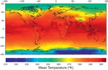
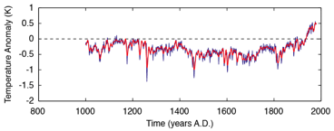
Here is how it works. A given millennial integration from a GCM is complete in both space and time. The figure at the top of this page is the mean temperature field from the ERIK2 GKSS ECHO-g millennial integration and clearly shows how all grid spaces in the field are available. Similarly, these model runs are also continuous over the full duration of the simulation. In the case of the ECHO-g simulation, the integration begins in 1000 C.E. and ends to 1990 C.E. The global mean time series for the ECHO-g simulation is shown in the figure below.
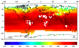
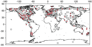
Given the complete set of information in the modeled climate field, the idea of a pseudoproxy experiment is to extract a small portion of the modeled data in a way that mimics the availability of proxy and instrumental data in the real world. This limited information is then used to reconstruct the known model values using modern reconstruction techniques, the results of which tell us how well our methodologies perform. The experiments typically involve four steps: (1) the complete GCM field is subsampled to mimic the availability of instrumental and proxy information in real-world climate reconstructions targeting the Common Era; (2) the time series that represent proxy information are perturbed to simulate the noise present in real-world proxies; (3) reconstruction algorithms are applied to the model-sampled pseudo “instrumental data” and pseudoproxy series to derive a reconstruction of the climate simulated by the GCM; and (4) the derived reconstruction is compared to the known model target. Each of these steps is an important part of the experimental design. As an example of the first step, the figures below show the grid box locations in the ECHO-g simulation that approximate the locations of the Mann et al. (1998) or Mann et al. (2008) multi-proxy networks and the data mask that is used to emulate the locations of the instrumental temperature grid boxes in the Brohan et al. (2006) dataset. The temporal duration of the pseudoproxies is taken over the whole simulation (in the case of the ECHO-g simulation this would be back to 1000 C.E.), while the instrumental data typically would be limited the interval from 1856 to 1980 C.E.
So what about the other steps? We will address the addition of noise to pseudoproxy networks in the next entry. Steps 3 and 4 are a longer story and comprise much of what our group studies. Various aspects of this work will be addressed in future entries that will attempt to outline what we have learned from pseudoproxy experiments and the implications of our results for real-world reconstructions of the climate of the Common Era.
***Update (2/2/2012): Please note my review on pseudoproxy experiments published in WIRES Climate Change:
Smerdon, J.E. (2012), Climate models as a test bed for climate reconstruction methods: pseudoproxy experiments, WIREs Clim. Change, 3:63-77, doi:10.1002/wcc.149.
Mean annual temperature field from the ERIK2 GKSS ECHO-g millennial integration (González-Rouco, 2006)
Map of grid box locations for pseudoproxy networks that approximate the Mann et al. (1998; red circles) or the Mann et al. (2008; black squares) multi-proxy networks. Time series from these locations would span the full duration of the millennial simulation.
Spatial data mask that approximates the available grid box locations in the Brohan et al. (2006) instrumental dataset. Time series from these locations would span the instrumental period (e.g. 1856-1980 C.E.).
Mean annual global temperature from the ERIK2 GKSS ECHO-g millennial integration (Gonzalez-Rouco, 2006). Annual values are shown in blue; low-pass filtered values (20-year period and below) are shown in red.

