The speed of sound increases with increases in temperature, salinity and pressure. Although the relationship is much more complex, to a first approximation, the following tables provides constant coefficients of change in sound speed for each of these parameters. Since changes in pressure in the sea typically result from changes in depth, values are provided with respect to changes in depth.

^[1]

Temperature has the largest effect on the speed of sound in the open ocean. Temperature variations range from 28 F near the poles to 90 F or more at the Equator. Of course, relevant temperature differences with regard to multibeam sonar systems are the variations that occur over relatively short distances, in particular those that occur with depth. These are discussed further below.

While the salinity of the world's oceans varies from roughly 32 to 38 ppt. These changes are gradual, such that within the range of a multibeam sonar, the impact on the speed of sound in the ocean is negligible. However near land masses or bodies of sea ice, salinity values can change considerably and can have significant effects on the way sound travels through water.

While the change in the speed of sound for a given depth change is small, in depth excursions where temperature and salinity are relatively constant, pressure changes as a result of increasing depth becomes the dominating factor in changes in the speed of sound.

The composite effects of temperature, salinity and pressure are measured in a vertical column of water to provide what is known as the "sound speed profile or SSP . A typical SSP is shown below:

Figure 2.1. Typical SSP

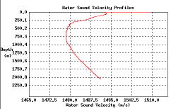
From the SSP above, one can see an iso-speed layer from the surface down to a few tens of meters due to mixing of water from wave action. This layer is called the "mixed surface layer" and is characterized by a flat or slightly negative (slanting down to the right) sound speed profile. The iso-speed layer is followed by a seasonal thermocline down to about 250 meters. Below, a larger main thermocline exists. These variations in the SSP are almost entirely due to changes in temperature of the water. Below the main thermocline, the temperature becomes largely constant and changes in pressure due to depth have the dominant effect on the SSP causing it to gradually increase.

In an effort to understand the effect on sonar performance of an incorrect sound speed at the keel, we must discuss the process of beam forming. This discussion surrounds a single simplified beam forming method, of which there are many. However it illustrates the effects well and the results can be applied to any sonar system.

The sound speed at the keel of the ship, local to the array, affects the directivity of the beams produced by the sonar. The result is that the sonar is not exactly looking in the direction we expect, introducing considerable error.

In multibeam sonar, a beam is formed by summing the sounds measured by multiple hydrophones time delayed by a specific amount with respect to each other. The following illustration depicts an array of hydrophones with an incident planar sound wave.

Figure 2.2. Diagram of Planar Soundwaves Orthogonally Incident on a Linear Hydrophone Array.

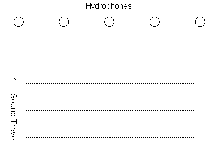
From this figure above, it is clear that the hydrophones will measure the incoming sounds simultaneously. However when the sound wave is incident from some angle , the hydrophones closer to the source will detect the sound prior to those farther away. Look at the figure below.

Figure 2.3. Diagram of Beam Forming Performed by A Linear Array

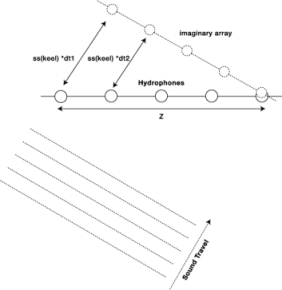
To listen in that direction, therefore, sonar systems sum the sounds measured from each hydrophone after delaying its measurement by the amount of time it would take for the sound to travel from the closest hydrophone. The result is an imaginary hydrophone array shown in the figure above, where the angle with respect to the actual array might be considered the direction the sonar beam is pointing. In this way, sounds coming from this direction are measured at each hydrophone in the imaginary array simultaneously.

As an example, assume the array is attempting to listen in a direction 30 degrees from its orientation. The sonar calculates the distance between the first hydrophone and the last hydrophone in the direction it is listening. This distance, X is simply

X = Z Sin (30)

The sonar divides the speed of sound at the keel into this distance X to get the time it will take the sound return to travel from the closer hydrophone to the further one.

t=X/ss

The measurements of the closer hydrophone are then summed with those of the further hydrophone delayed by this interval such that the arrival of the sound signal at the last hydrophone coincides with the delayed measurement of this closer hydrophone.

If the sound speed used to calculate this delay time is too low, the calculated delay time will be too large. A larger delay time results in a beam that is pointed further away from orthogonal than has been assumed.

If all this is confusing, just try to remember:

SS(Keel) Too Low - > Beam Fan Pattern Too Wide

SS(Keel) Too High - > Beam Fan Pattern Too Narrow

It is important to realize that the beam perpendicular to the plane of the sonar array is directionally unaffected. Only the beams formed by delaying the signals from individual hydrophones look in the wrong direction when the speed of sound at the keel is in error. This implies, of course, that the effect a sound speed error has on any given data set are largely dependent on the orientation of the installed sonar.

Many sonar arrays are installed flush with the hull of the ship and parallel to the sea (nominal) floor. A sonar array installed parallel to the sea floor sees little or no error in the nadir beam due to errors in the keel sound speed. However, because of the high beam angles at the outer beams, the errors are exacerbated at the edges of the swath. When the value is too low, the beam fan shape is erroneously wide, causing the measured bathymetry at the outer beams to be too deep. (Sound travel times are erroneously longer for the wider beams.) This causes the cross track shape of a swath to "frown". The converse is true, of course, for keel sound speeds that are too high.

Other sonar arrays are installed on a V-shaped structure mounted to the bottom of the ship or towfish. For these sonars, the zero angle beam, whose direction is unaffected by the keel sound speed, is that which is formed perpendicular to the array at some angle from nadir. The effect on the beam pattern, is the same - keel sound speed too low -> beam pattern is too wide - keel sound speed too high -> beam pattern too narrow. However, in this case, the effects on the data set are slightly different. A wider beam pattern does indeed cause erroneously deep bathymetry values at the beams furthest from the ship's track, but the beams directly beneath the ship will be erroneously shallow. Similarly, a narrower beam pattern causes erroneously shallow bathymetry values at beams furthest from the ship's track and erroneously deep values directly beneath the ship.

In both sonar installation orientations positive keel sound speed errors result in "frowns" in the cross track swath profile, while negative errors result in "smiles". The distinction to make is that the beams unaffected by these errors are beneath the ship for the former and at an angle orthogonal to the sonar array for the latter.

One final effect to point out. Multibeam sonars use beam forming both for projection as well as for reception of sound pulses. Moreover, beam forming is done, not only in the athwartships direction to create a swath, but fore and aft to increase measurement resolution. Typically the beam footprint created by the projectors on the sea floor is large compared to that created by the receivers. In this way, errors in the receive footprint still fall within that of the projection footprint. However significant sound speed errors at the keel can upset this balance lowering the signal to noise ratio of the sonar and compromising data quality.

Here's the kicker. ERRORS IN KEEL SOUND SPEED ARE (typically) NOT RECOVERABLE! Let us say that again:

Because sonar systems do not save wave forms from individual hydrophones, one cannot go back and apply corrected sound speed values to beam forming calculations. This value must be correct the first time. Therefore, and it cannot be stressed enough, sonar operators must always be conscience of the correct operation of any device that provides the keel sound speed measurement to the sonar.

Bathymetric sonar systems calculate water depths by measuring the time it takes a sound pulse to travel to the bottom and back to the receiver. To translate these time measurements into distances, one must know the speed at which sound travels through water and the general trajectory the sound traveled. As we have seen, temperature, pressure, and salinity all contribute to the speed of sound in water. Moreover, differences in sound speed across the water column acts as a lens bending the path that sound travels. For these reasons, it is imperative to have accurate sound speed profiles for any data set.

Inaccurate sound speed profiles may be the single largest correctable cause of bathymetry errors in multibeam sonar data. Understanding the various effects errors in sound speed can have on sonar data is challenging and deserves careful consideration. Even more difficult, is recognizing these errors from other sources of error in the data. A solid theoretical understanding is essential.

Errors in the sound speed profile produce predictable, although often confused, results in the data.

For example, a simple step offset in the sound speed profile will cause the calculated bathymetry to be shallower for higher sound speeds, and deeper for lower sound speeds. Not so obvious, is that relative changes in sound speed down through the water column cause sound to bend, a process called refraction. Therefore, errors in the relative changes in sound speed through the water column cause errors in the calculated sound trajectory. Because the bending is larger for sound traveling at oblique angles to the gradient, oblique beams (usually the outer ones) have more error. All of this is further complicated by the fact that sound speed profile errors high in the water column can exacerbate or offset the effects of those lower in the water column.

2.1.2.2.1. Refraction

It is convenient, when talking about sound and its travel path from a point, to consider the path as a ray. This is a common technique in wave theory, used in optics and other sciences. In a homogeneous medium sound does indeed travel in a straight line. However, when a sound wave passes between two mediums having different sound speeds its direction is bent. This is a property of waves more than sound itself, and many theories and explanations, with varying degrees of success, have been put forth over they years. While not true in all cases a simple one for illustration is offered here.

Figure 2.4. Snell's Law

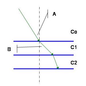
Consider sound wave incident on a boundary between two bodies of water having differing sound speeds as shown in the figure above. Snell's Law states that the Cosine of the initial angle of incidence divided by the initial sound speed is a constant as the sound passes from regions of differing sound speeds.

Cos (A)/ Co = Constant

Therefore, if the new region has lower sound speed, the Cosine of the angle of incidence must be less than that of the previous region. Hence the new angle of incidence is less. So one might imagine the sound bending "toward" regions of lower sound speed, in the sense that the angle of sound travel is more steep, and "away" from regions of higher sound speed in the sense that the angle of incidence is more shallow.

Then if one knows the angle that a sound wave left its source, and the sound speed profile of the medium it passes through, one can calculate the path the wave takes over its entire trip.

A slightly more complicated example is one where the sound speed of a single medium changes linearly with depth rather than at discrete depth intervals. In this scenario, the sound ray bends continuously over its travel path. It can be shown that the path the sound travels is that of the arc of a circle whose radius, R, is the ratio of the initial sound speed and the slope of the gradient (R = Co/g).^[2]

This process, of calculating the course of travel of a sound ray through a water column of varying sound speed, is called "ray tracing" and is essential to sonar performance. Since sound does not travel as a straight line though the ocean, sonar systems must calculate propagation paths for both the the ping and return to calculate the correct distance and direction of the reflecting object.